

SAT: Formulate, Embed, and Submit#
The example of the SAT: a Simple Objective section formulates an objective function for a simple SAT problem. The D‑Wave quantum computer is also well suited to solving optimization problems with binary variables. Real-world optimization problems often come with constraints: conditions of the problem that any valid solution must satisfy.
For example, when optimizing a traveling salesperson’s route through a series of cities, you need a constraint forcing the salesperson to be in exactly one city at each stage of the trip: a solution that puts the salesperson in two or more places at once is invalid.
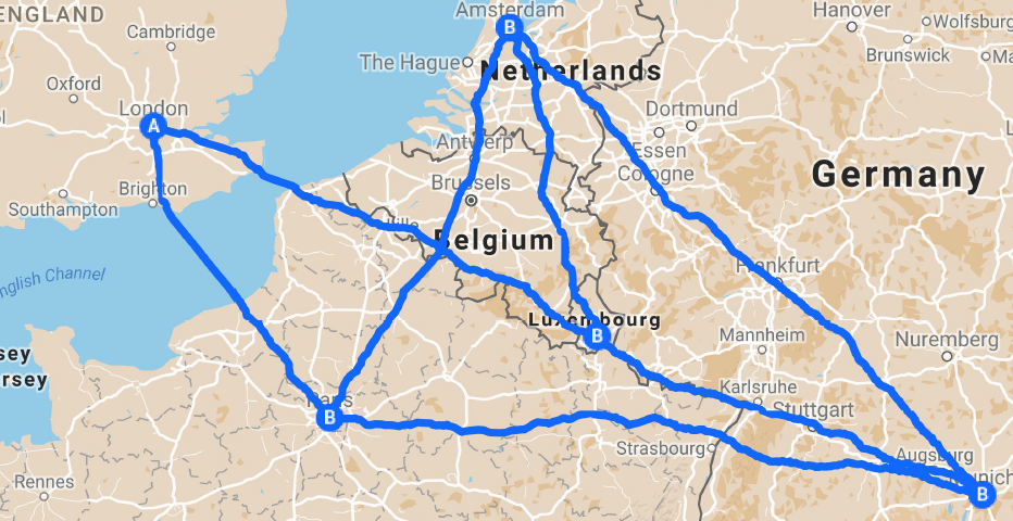
Fig. 61 The traveling salesperson problem is an optimization problem that can be solved using exactly-one-true constraints. Map data © 2017 GeoBasis-DE/BKG (© 2009), Google.#
In fact, the example of the SAT: a Simple Objective section is actually also an example of a simple constraint, the equality (or XNOR) constraint. The example of this section is slightly more complex. The exactly-one-true constraint is the Boolean satisfiability problem of finding, given a set of variables, when exactly one variable is TRUE (equals 1). This example looks at an exactly-one-true constraint for three variables.
The problem-solving process is the same as described in the QUBOs and Ising Models section.
Note
Quantum samplers optimize objective functions that represent problems in formats that are unconstrained (e.g., QUBOs, or unconstrained binary optimization problems). As is shown in this section, any constraints in the original problem are represented as part of the objective function; this technique is known as penalty models.
In addition, some of the Leap service’s quantum-classical hybrid solvers accept only unconstrained objective functions; for example, hybrid BQM solvers. Thus, for these solvers any constraints must be added to the objective function, typically as a penalty. However, some of the Leap service’s hybrid solvers can handle constraints natively, as shown in the Basic Hybrid Examples examples. For more information, see the Get Started with Optimization section.
Formulating an Objective Function#
For problems with a small number of binary variables (in this example three: \(a\), \(b\), and \(c\)), you can tabulate all the possible permutations and identify the states when exactly one variable is 1 and the other two are 0. You do so with a truth table:
\(a\) |
\(b\) |
\(c\) |
Exactly One is True |
|---|---|---|---|
0 |
0 |
0 |
FALSE |
1 |
0 |
0 |
TRUE |
0 |
1 |
0 |
TRUE |
1 |
1 |
0 |
FALSE |
0 |
0 |
1 |
TRUE |
1 |
0 |
1 |
FALSE |
0 |
1 |
1 |
FALSE |
1 |
1 |
1 |
FALSE |
Notice that the three constraint-satisfying states in the truth table have in common that the sum of variables equals \(1\), so you can express the constraint mathematically as the equation,
As noted in the QUBOs and Ising Models section, you can solve some equations by minimization if you formulate an objective function that takes the square[1] of the subtraction of one side from another:
Expanding the squared term—while remembering that for binary variables with values 0 or 1 the square of a variable is itself, \(X^2 = X\)—shows in explicit form the objective function’s quadratic and linear terms.
Notice that this objective formula matches the QUBO format for three variables,
where \(a_i=-1\) and \(b_{i,j}=2\), with a difference of the \(+1\) term.[2]
Below, the truth table is shown with an additional column of the energy for the objective function found above. The lowest energy states (best solutions) are those that match the exactly-one-true constraint.
\(a\) |
\(b\) |
\(c\) |
Exactly One is True |
Energy |
|---|---|---|---|---|
0 |
0 |
0 |
FALSE |
1 |
1 |
0 |
0 |
TRUE |
0 |
0 |
1 |
0 |
TRUE |
0 |
1 |
1 |
0 |
FALSE |
1 |
0 |
0 |
1 |
TRUE |
0 |
1 |
0 |
1 |
FALSE |
1 |
0 |
1 |
1 |
FALSE |
1 |
1 |
1 |
1 |
FALSE |
4 |
Clearly, a solver minimizing the objective function \(2ab + 2ac + 2bc - a - b - c\) can be expected to return solutions (values of variables \(a, b, c\)) that satisfy the original problem of an exactly-one-true constraint.
As explained in the SAT: a Simple Objective example, to solve a QUBO with a D‑Wave quantum computer, you must map (minor embed) it to the QPU. That step is explained in detail in the next section.
Minor Embedding#
This section explains how the QUBO created in the previous section is minor-embedded onto a QPU, in this case, an Advantage QPU with its Pegasus graph.
D‑Wave provides automatic minor-embedding tools, and if you are submitting your problem to a Leap service’s quantum-classical hybrid solver, the solver handles all interactions with the QPU.
The QUBO developed for an exactly-one-true constraint with three variables in the previous section, \(2ab + 2ac + 2bc - a - b - c\), can be represented by the triangular graph shown in Figure 62.
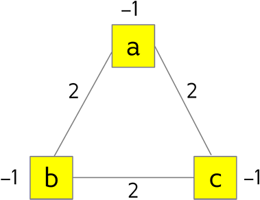
Fig. 62 Triangular graph for an exactly-one-true constraint with its biased nodes and edges.#
As explained in the Minor Embedding section, nodes that represent the objective function’s variables such as \(a\) are mapped to qubits on the QPU while edges that represent the objective function’s quadratic terms such as \(ab\) are mapped to couplers.
Figure 63 shows such a mapping, between the graph representing the QUBO on the left and one particular minor-embedding on the right. (Rerunning Ocean software’s minorminer tool, which produced this minor embedding, generates embeddings to various qubits across the QPU; the particular qubit numbers noted here are unimportant.)
Nodes \(a, b, c\) (grey circles in the left-hand panel) map to qubits \(1812, 5169, 1827\) (blue circles in the right-hand panel), respectively.
Edges \(ab, bc, ca\) (orange lines in the left-hand panel) map to couplers \([1812, 5619], [1827, 5619], [1812, 1827]\) (blue lines in the right-hand panel), respectively.
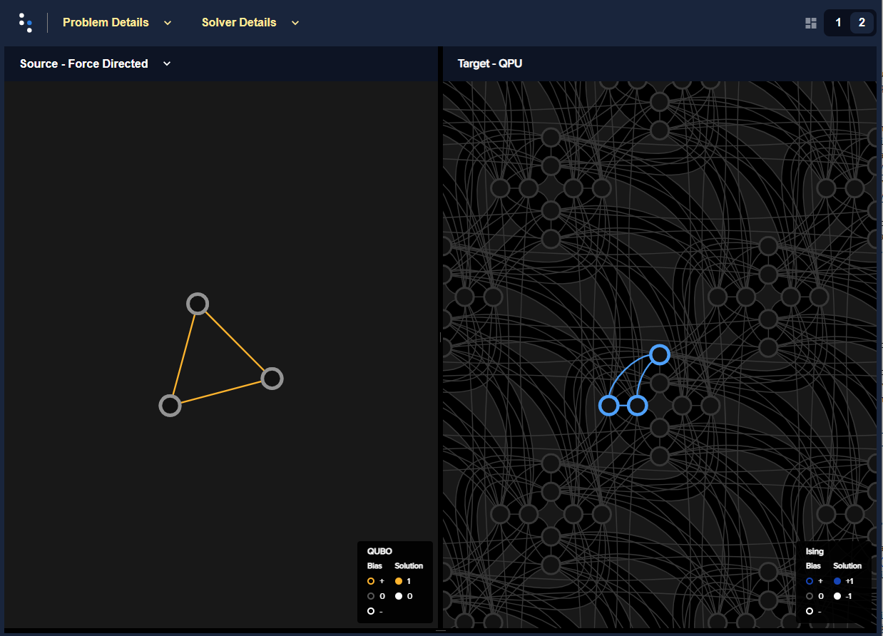
Fig. 63 Embedding in the Pegasus topology for an exactly-one-true constraint rendered by Ocean software’s problem inspector. The original QUBO is represented on the left and its embedded representation on the right.#
But, as the Topologies section notes, D‑Wave QPUs are not fully connected. For larger graphs than the example above, you may not always be able to map each node to a qubit and find connecting couplers to represent all edges.
How are more complex graphs minor-embedded? Minor embedding often requires chains.
Chains#
To understand how chaining qubits overcomes the problem of sparse connectivity, consider minor embedding the triangular graph of Figure 62 into two target graphs, one sparser than the other. Figure 64 shows two such embeddings: the triangular graph is mapped on the left to a fully-connected graph of four nodes (called a \(K_4\) complete graph) and on the right to a sparser graph, also of four nodes. For the left-hand embedding, you can choose any mapping between \(a, b, c\) and \(0, 1, 2, 3\); here \(a, b, c\) are mapped to \(2, 0, 1\), respectively. For the right-hand embedding, however, no choice of just three target nodes suffices. The same \(2, 0, 1\) target nodes leaves \(b\) disconnected from \(c\). Chaining target nodes \(0\) and \(3\) to represent node \(b\) makes use of both the connection between \(0\) to \(2\) and the connection between \(3\) and \(1\).
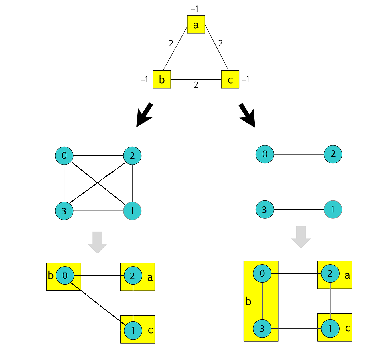
Fig. 64 Embedding a triangular graph into fully connected and sparse four-node graphs.#
On QPUs, chaining qubits is accomplished by setting the strength of their connecting couplers negative enough to strongly correlate the states of the chained qubits; if at the end of most anneals these qubits are in the same classical state, representing the same binary value in the objective function, they are in effect acting as a single variable.
As an example, consider a fully-connected graph of five nodes (a \(K_5\) graph). Such a graph cannot be mapped to five qubits of an Advantage QPU because the Pegasus graph’s connectivity is too sparse. Instead, some nodes are mapped to chains of qubits.
Figure 65 shows a \(K_5\) graph of some arbitrary problem on the left and a minor-embedding on the right. Here, variable 3 (highlighted magenta) is represented by a two-qubit chain of qubits 4408 and 2437 (highlighted magenta) while variables 0, 1, 2, and 4 are represented by single qubits 4333, 4348, 2497, and 2512.
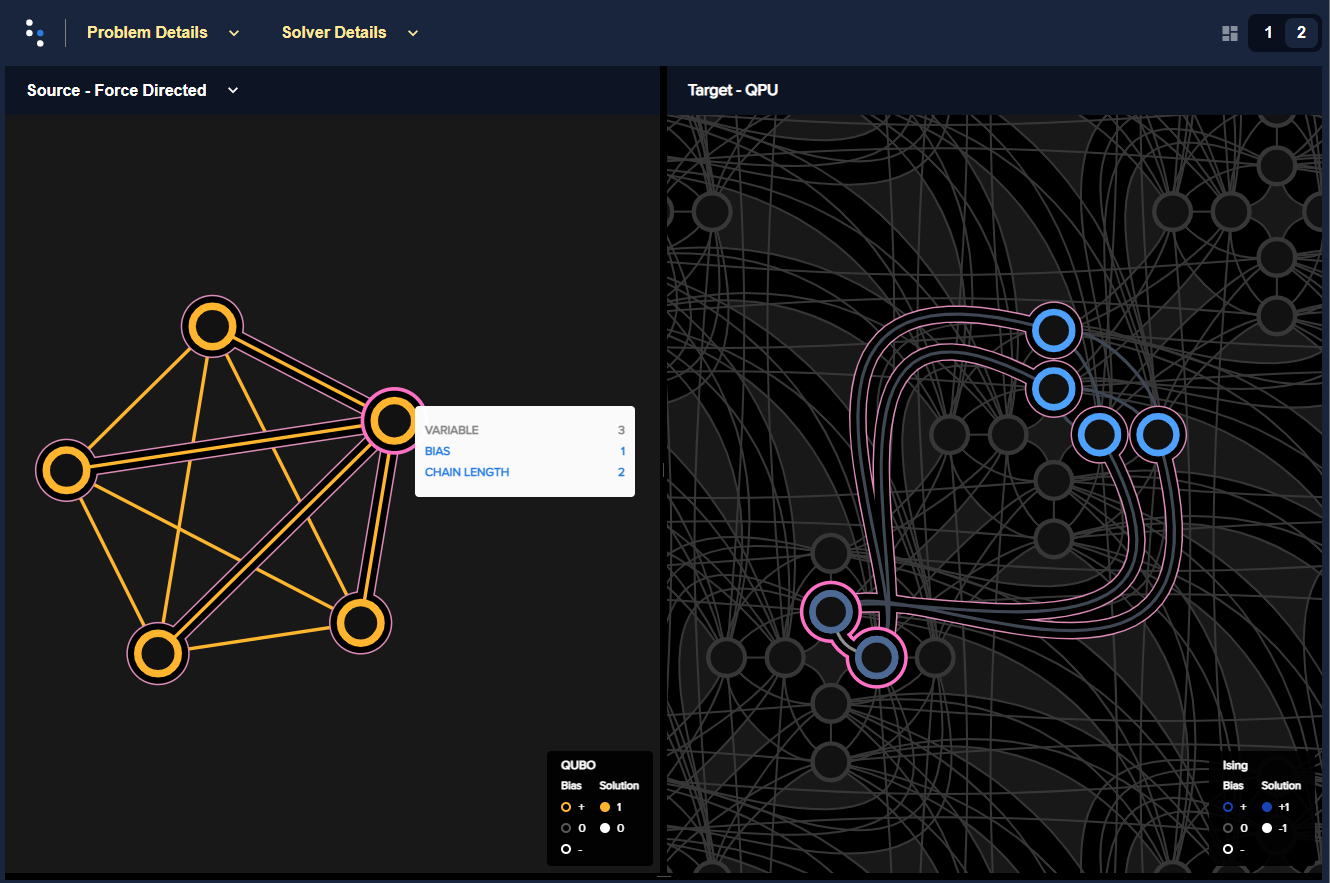
Fig. 65 Embedding for a \(K_5\) fully connected graph in the Pegasus topology rendered by Ocean software’s problem inspector. The original QUBO is represented on the left and its embedded representation, with its two-qubit chain, on the right.#
Manual Minor-Embedding#
Manually minor-embedding a problem is typically undertaken only for problems that have either very few variables or a repetitive structure that maps to unit cells of the QPU topology—in both cases you work with one or more unit cells. Additionally, you might make minor adjustments to an embedding found by software. You are unlikely to manually embed a random 100-variable problem.
This section provides an example of how you can calculate the biases needed for minor-embedding on a simple problem. Ocean software’s minor-embedding tools, such as minorminer, do similar calculations.
Example of Manual Minor Embedding
This example returns to the QUBO developed for an exactly-one-true constraint with three variables in the Formulating an Objective Function section above, \(2ab + 2ac + 2bc - a - b - c\), as represented by the triangular graph shown in Figure 62 above. For simplicity, it is minor-embedded into a Chimera graph.
To see how a triangular graph fits on the Chimera graph, take a closer look at the unit cell in the Chimera topology shown in Figure 66. Notice that there is no way to make a triangular closed loop of three qubits and their connecting edges. However, you can make a closed loop of four qubits and their edges using, say, qubits 0, 1, 4, and 5.
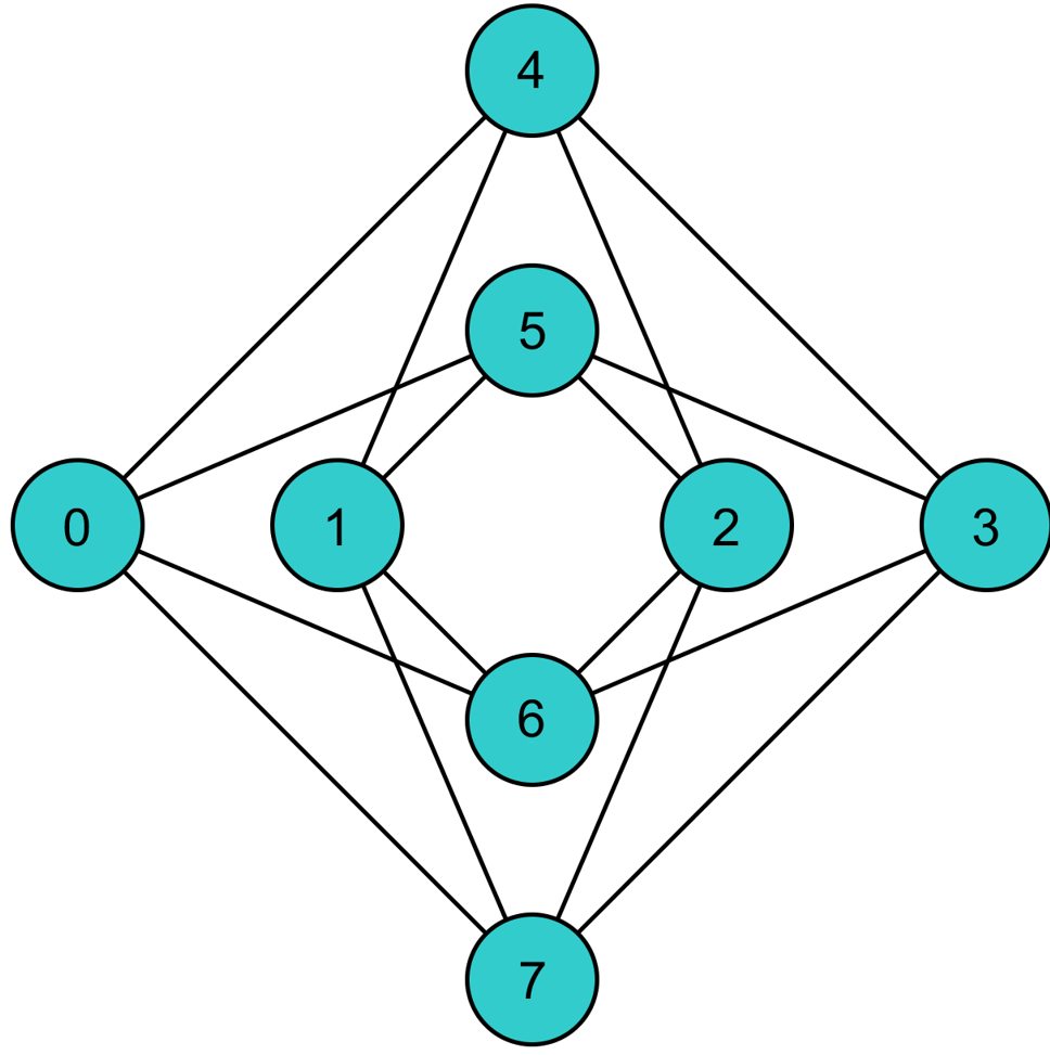
Fig. 66 Unit cell in the Chimera topology.#
As in the example of the Chains section, make a three-node loop of a four-node structure by representing a single variable with a chain of two qubits. Figure 67 shows a chaining of qubit 0 and qubit 5 to represent variable \(b\).
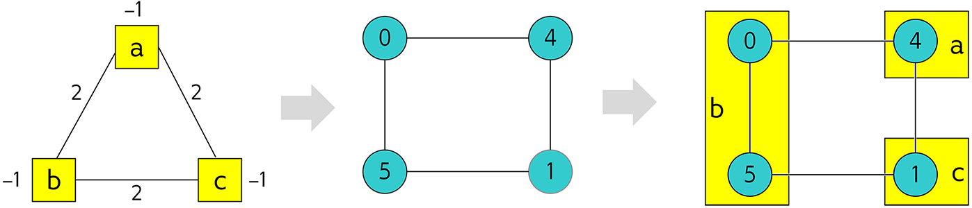
Fig. 67 Embedding a triangular graph into the Chimera graph by using a chain.#
Here, for qubits 0 and 5 to represent variable \(b\), the strength of the coupler between them must be set negative enough.
The mapping of Figure 67 is straightforward for non-chained qubits with biases being the linear coefficients of the objective function and coupler strengths the quadratic coefficients:
Variables \(a\) and \(c\), represented by qubits 4 and 1, respectively, have bias \(-1\).
Edges \((a,b), (a,c), (b,c)\), represented by couplers \((0,4), (1,4), (1,5)\), respectively, have strengths \(2\).
To chain qubits 0 and 5 to represent variable \(b\) requires that you add a strong negative coupling strength between them. This coupling has no corresponding quadratic coefficient in the objective function, so other biases must be adjusted to compensate. This process requires a few steps:
Evenly split the bias of \(-1\) from variable \(b\) between qubits 0 and 5. Now the bias of these two qubits is \(-0.5\).
Choose a strong negative coupling strength for the chain between qubits 0 and 5. This example arbitrarily chooses \(-3\) because it is stronger than the values for couplers around it.[3]
Compensate for the \(-3\) added in step 2 by adding \(-\frac{-3}{2} = 1.5\) to each bias of qubits 0 and 5. Now the biases for these qubits are \(1\).
The resulting minor-embedding values are shown in the tables below.
Node |
Linear Coefficient |
Qubits |
Bias |
|---|---|---|---|
a |
-1 |
4 |
-1 |
b |
-1 |
0, 5 |
1, 1 |
c |
-1 |
1 |
-1 |
Edge |
Quadratic Coefficient |
Coupler |
Strength |
|---|---|---|---|
(a,b) |
2 |
(0,4) |
2 |
(a,c) |
2 |
(1,4) |
2 |
(b,c) |
2 |
(1,5) |
2 |
(0,5) |
-3 |
You program the quantum computer to solve this problem by configuring the QPU’s qubits with these biases and its couplers with these strengths.
Note
When using the QUBO formulation, as in this example, you compensate for the quadratic term a chain introduces into the objective by adding its negative, divided by the number of qubits in the chain, to the biases of the chain’s qubits; this compensation is not used for the Ising formulation, where the the energies of valid solutions are simply shifted by the introduced quadratic term.
The solutions returned from the QPU express the states of qubits at the end of each anneal. To translate qubit states to values of the problem variables, the solutions must be unembedded.
For example, consider the following results for 1000 anneals:
Energy |
Qubit |
Occurrences |
|||
|---|---|---|---|---|---|
0 |
5 |
4 |
1 |
||
-1.0 |
0 |
0 |
1 |
0 |
206 |
-1.0 |
0 |
0 |
0 |
1 |
526 |
-1.0 |
1 |
1 |
0 |
0 |
267 |
0.0 |
1 |
1 |
0 |
1 |
1 |
For this simple example with its single chain, unembedding consists of mapping qubits 4, 1 to variables \(a, c\), and qubits 0, 5 to variable \(b\). The results in the table above unembedded to:
Row 1: Solution \((a, b, c) = (1, 0, 0)\) with energy \(-1\) was found 206 times.
Row 2: Solution \((a, b, c) = (0, 0, 1)\) with energy \(-1\) was found 526 times.
Row 3: Solution \((a, b, c) = (0, 1, 0)\) with energy \(-1\) was found 267 times.
One anneal ended with result \((a, b, c) = (0, 1, 1)\), which is not a correct solution, and has a higher energy than the correct solutions.
Note
Notice also that the energy of the valid solutions, the ground-state energy, is \(-1\), not the zero calculated in the Formulating an Objective Function section’s truth table. This is because of the constant \(+1\) dropped from the objective function, \(E(a,b,c) = 2ab + 2ac + 2bc - a - b - c + 1\).
The next section shows how you submit a problem to a D‑Wave quantum computer.
Submitting#
This section uses D‑Wave’s open-source Ocean SDK to submit the exactly-one-true problem formulated in the previous subsections.
Before you can submit a problem to D‑Wave solvers, you must have an account and an API token; visit the Leap service to sign up for an account and get your token.
Note
To run the following steps yourself requires prior configuration of some requisite information for problem submission through SAPI. If you have installed the Ocean SDK or are using a supported IDE, this is typically done as a first step.
For more information, including on Ocean SDK installation instructions and detailed examples, see the Ocean software documentation.
The Ocean software can heuristically find minor-embeddings for your QUBO or Ising objective functions, as shown here.
First, select a quantum computer. Ocean software provides
feature-based solver selection,
enabling you to select a quantum computer that meets your requirements on its
number of qubits, topology, particular features, etc. This example, uses the
default.
from dwave.system import DWaveSampler, EmbeddingComposite
sampler = EmbeddingComposite(DWaveSampler())
Set values of the QUBO and submit to the selected QPU.
linear = {('a', 'a'): -1, ('b', 'b'): -1, ('c', 'c'): -1}
quadratic = {('a', 'b'): 2, ('b', 'c'): 2, ('a', 'c'): 2}
Q = {**linear, **quadratic}

sampleset = sampler.sample_qubo(Q, num_reads=5000)
Below are results from running this problem on a Advantage system:
>>> print(sampleset)
   a  b  c energy num_oc. chain_b.
0  0  0  1   -1.0    1591     0.0
1  1  0  0   -1.0    2040     0.0
2  0  1  0   -1.0    1365     0.0
3  1  0  1    0.0       2     0.0
4  1  1  0    0.0       1     0.0
5  0  1  1    0.0       1     0.0
['BINARY', 6 rows, 5000 samples, 3 variables]
In the results of 5000 reads, you see that the lowest energy occurs for the three valid solutions to the problem.