

NOT Gate: Simple QUBO#
This example solves a simple problem of a Boolean NOT gate to demonstrate the mathematical formulation of a problem as a binary quadratic model (BQM) and using Ocean software to solve such problems on a D‑Wave quantum computer. Other examples demonstrate the more-advanced steps that are typically needed for solving actual problems.
Example Requirements#
The code in this example requires that your development environment have Ocean software and be configured to access SAPI, as described in the Configuring Access to the Leap Service (Basic) section.
Solution Steps#
Basic Workflow: Formulation and Sampling describes the problem-solving workflow as consisting of two main steps: (1) Formulate the problem as an objective function in a supported model and (2) Solve your model with a D‑Wave solver.
This example mathematically formulates the BQM and uses Ocean tools to solve it on a D‑Wave quantum computer.
Formulate the NOT Gate as a BQM#
You use a sampler like the D‑Wave quantum computer to solve binary quadratic models (BQM)[2]: given \(M\) variables \(x_1,...,x_N\), where each variable \(x_i\) can have binary values \(0\) or \(1\), the quantum computer tries to find assignments of values that minimize
where \(q_i\) and \(q_{i,j}\) are configurable (linear and quadratic) coefficients. To formulate a problem for a D‑Wave quantum computer is to program \(q_i\) and \(q_{i,j}\) so that assignments of \(x_1,...,x_N\) also represent solutions to the problem.
Ocean tools can automate the representation of logic gates as a BQM, as demonstrated in the example of the Logic Circuit: Embedding Effects section.
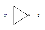
Fig. 71 A NOT gate.#
Representing the Problem With a Penalty Function#
This example demonstrates a mathematical formulation of the BQM. As explained in the Penalty Models section, you can represent a NOT gate, \(z \Leftrightarrow \neg x\), where \(x\) is the gate’s input and \(z\) its output, using a penalty function:
This penalty function represents the NOT gate in that for assignments of variables that match valid states of the gate, the function evaluates at a lower value than assignments that would be invalid for the gate.[1] Therefore, when the D‑Wave quantum computer minimizes a BQM based on this penalty function, it finds those assignments of variables that match valid gate states.
Formulating the Problem as a QUBO#
Sometimes penalty functions are of cubic or higher degree and must be reformulated as quadratic to be mapped to a binary quadratic model. For this penalty function you just need to drop the freestanding constant: the function’s values are simply shifted by \(-1\) but still those representing valid states of the NOT gate are lower than those representing invalid states. The remaining terms of the penalty function,
are easily reordered in standard QUBO formulation:
where \(z=x_2\) is the NOT gate’s output, \(x=x_1\) the input, linear coefficients are \(q_1=q_2=-1\), and quadratic coefficient is \(q_{1,2}=2\). These are the coefficients used to program a D‑Wave quantum computer.
Often it is convenient to format the coefficients as an upper-triangular matrix:
See the Reformulating a Problem section for more information about formulating problems as QUBOs.
Solve the Problem by Sampling#
Now solve on a D‑Wave quantum computer using the
DWaveSampler sampler from Ocean software’s
dwave-system package. Also use its
EmbeddingComposite composite to map the
unstructured problem (variables such as \(x_2\) etc.) to the sampler’s
graph structure (the QPU’s numerically indexed qubits)
in a process known as minor-embedding.
The next code sets up a D-Wave quantum computer as the sampler.
Note
The following code sets a sampler without specifying SAPI parameters. Configure a default solver, as described in the Configuring Access to the Leap Service (Basic) section, to run the code as is, or see the dwave-cloud-client tool on how to access a particular solver by setting explicit parameters in your code or environment variables.
>>> from dwave.system import DWaveSampler, EmbeddingComposite
>>> sampler = EmbeddingComposite(DWaveSampler())
Because the sampled solution is probabilistic, returned solutions may differ between runs. Typically, when submitting a problem to the system, you ask for many samples, not just one. This way, you see multiple “best” answers and reduce the probability of settling on a suboptimal answer. Below, ask for 5000 samples.
>>> Q = {('x', 'x'): -1, ('x', 'z'): 2, ('z', 'x'): 0, ('z', 'z'): -1}
>>> sampleset = sampler.sample_qubo(Q, num_reads=5000, label='SDK Examples - NOT Gate')
>>> print(sampleset)
   x  z energy num_oc. chain_.
0  0  1   -1.0    2266     0.0
1  1  0   -1.0    2732     0.0
2  0  0    0.0       1     0.0
3  1  1    0.0       1     0.0
['BINARY', 4 rows, 5000 samples, 2 variables]
Almost all the returned samples represent valid value assignments for a NOT gate, and minima (low-energy states) of the BQM, and with high likelihood the best (lowest-energy) samples satisfy the NOT gate formulation:
>>> sampleset.first.sample["x"] != sampleset.first.sample["z"]
True
Summary#
In the terminology of the Ocean Software Stack section, Ocean tools moved the original problem through the following layers:
The sampler API is a QUBO formulation of the problem.
The sampler is the
DWaveSamplerclass sampler.The compute resource is a D‑Wave quantum computer.