Basic Workflow: Formulation and Sampling

This section provides a high-level description of how you solve problems using quantum computers directly. For solving problems with hybrid solvers, see the Basic Workflow: Models and Sampling section.

The two main steps of solving problems using quantum computers are:

1. Formulate[1] your problem as an objective function

   An objective function (cost function) is a mathematical expression of the problem to be optimized; for quantum computing, these are quadratic models and (for some hybrid solvers) nonlinear models that have lowest values (energy) for good solutions to the problems they represent.

2. Find good solutions by sampling

   Samplers are processes that sample from low-energy states of objective functions. Find good solutions by submitting your model to one of a variety of D-Wave’s quantum, classical, and hybrid quantum-classical samplers.

Fig. 37 Solution steps: (1) a problem known in “problem space” (a circuit of Boolean gates, a graph, a network, etc) is formulated as a model, mathematically or using Ocean functionality, and (2) the model is sampled for solutions.

[1]

For quantum computing, as for classical, solving a problem requires that it be formulated in a way the computer and its software understand. For example, if you want your laptop to calculate the area of a $1 coin, you might express the problem as an equation, \(A=\pi r^2\), that you program as math.pi*13.245**2 in your Python terminal. For a laptop with Python software, this formulation—a particular string of alphanumeric symbols—causes the manipulation of bits in a CPU and memory chips that produces the correct result.

Objective Functions

To express a problem for a D-Wave solver in a form that enables solution by minimization, you need an objective function, a mathematical expression of the energy of a system. When the solver is a QPU, the energy is a function of binary variables representing its qubits[2]; for quantum-classical hybrid solvers, the objective function might be more abstract[3].

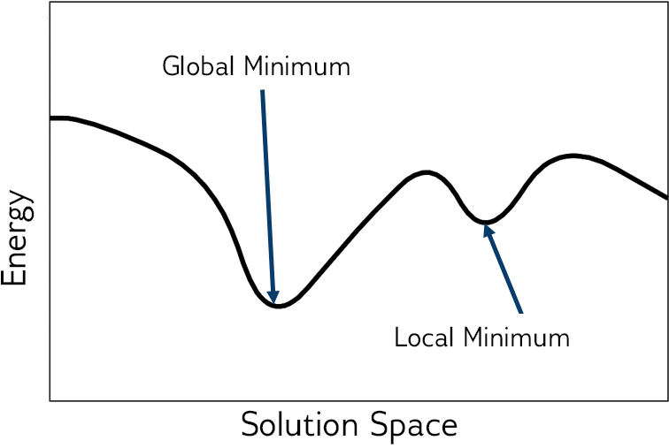
Fig. 38 Energy of the objective function.

For most problems, the lower the energy of the objective function, the better the solution. Sometimes any low-energy state is an acceptable solution to the original problem; for other problems, only optimal solutions are acceptable. The best solutions typically correspond to the global minimum energy in the solution space; see the figure above.

There are many ways of mapping between a problem—chains of amino acids forming 3D structures of folded proteins, traffic in the streets of Beijing, circuits of binary gates—and an objective function to be solved (by sampling) with a D-Wave quantum computer, hybrid solver, or locally on your CPU. The Basic QPU Examples and Basic Hybrid Examples show some simple objective functions to help you begin.

For more detailed information on objective functions, how D-Wave quantum computers minimize objective functions, see the What is Quantum Annealing? section; for techniques for reformulating problems as objective functions, see the Reformulating a Problem section.

For code examples that formulate models for various problems, see D-Wave’s examples repo and many example customer applications on the D-Wave website.

[2]

If you are solving your problem directly on a D-Wave quantum computer, the system is the qubits of a quantum processing unit (QPU) and your objective function represents the states of the qubits as binary variables, and the physical biases and couplings applied to these qubits as, respectively, linear and quadratic coefficients. By formulating an objective function such that lowest energy states represent good solutions to your problem, you can solve your problem by minimizing the objective function. In the case of a D-Wave quantum computer, the QPU uses quantum annealing to seek the minimum of the energy landscape for its qubits with the biases and couplings applied by your objective function.

[3]

For hybrid solvers, some parts of the objective function are minimized using classical heuristics and some by the QPU.

Simple Objective Example

As an illustrative example, consider solving a simple equation, \(x+1=2\), not by the standard algebraic techniques but by formulating an objective that at its minimum value assigns a value to the variable, \(x\), that is also a good solution to the original equation.

Taking the square of the subtraction of one side from another, you can formulate the following objective function to minimize:

\[ \begin{align}\begin{aligned}\text{E}(x) &= [2-(x+1)]^2\\&= (1-x)^2\end{aligned}\end{align} \]

In this case minimization, \(\min_x{(1-x)^2}\), seeks the shortest distance between the sides of the original equation, which occurs at equality (with the square eliminating negative distance).

The Simple Sampling Example example below shows an equally simple solution by sampling.

Supported Models

To express your problem as an objective function and submit to a D-Wave sampler for solution, you typically use one of the Ocean software quadratic[4] models supported by D-Wave quantum computers:

• Binary quadratic models (BQM) are unconstrained and typically represent problems of decisions that could either be true (or yes) or false (no); for example, should an antenna transmit, or did a network node fail? The model uses \(0/1\)-valued variables and \(-1/1\)-valued variables; constraints are typically represented as penalty models.

• Ising models are unconstrained and typically represent problems of decisions that could either be true or or false. The model uses \(-1/1\)-valued variables; constraints are typically represented as penalty models.

• QUBOs are unconstrained and typically represent problems of decisions that could either be true or false. The model uses \(0/1\)-valued variables; constraints are typically represented as penalty models.

[4]

Quadratic functions have one or two variables per term. A simple example of a quadratic function is,

\[D = Ax + By + Cxy\]

where \(A\), \(B\), and \(C\) are constants. Single variable terms—\(Ax\) and \(By\) here—are linear with the constant biasing the term’s variable. Two-variable terms—\(Cxy\) here—are quadratic with a relationship between the variables.

Ocean software also provides support for higher order models, which are typically reduced to quadratic for sampling.

Samplers

Samplers are processes that sample from low-energy states of objective functions. Having formulated an objective function that represents your problem (typically as a quadratic or nonlinear model), you sample it for solutions.

D-Wave provides quantum, classical, and quantum-classical hybrid samplers that run either remotely (for example, in D-Wave’s Leap service) or locally on your CPU.

• QPU Solvers

  D-Wave currently supports Advantage quantum computers.

• Quantum-Classical Hybrid Solvers

  Quantum-classical hybrid is the use of both classical and quantum resources to solve problems, exploiting the complementary strengths that each provides. For an overview of, and motivation for, hybrid computing, see: Medium Article on Hybrid Computing.

  D-Wave provides two types of hybrid solvers: Leap service’s hybrid solvers, which are cloud-based hybrid compute resources, and hybrid solvers developed in Ocean software’s dwave-hybrid tool.

• Classical Solvers

  You might use a classical solver while developing your code or on a small version of your problem to verify your code.

  For information on classical solvers, see the Classical Solvers section.

Simple Sampling Example

As an illustrative example, consider solving by sampling the objective, \(\text{E}(x) = (1-x)^2\) found in the Simple Objective Example subsection above to represent equation, \(x+1=2\).

This example creates a simple sampler that generates 10 random values of the variable \(x\) and selects the one that produces the lowest value of the objective:

>>> import random
...
>>> x = [random.uniform(-10, 10) for i in range(10)]
>>> e = list(map(lambda x: (1-x)**2, x))
>>> best_found = x[e.index(min(e))]

One particular execution found this best solution:

>>> print('x_i = ' + ' , '.join(f'{x_i:.2f}' for x_i in x))     
x_i = 7.87, 1.79, 9.61, 2.37, 0.68, -2.93, 3.96, 1.30, -3.85, -0.13
>>> print('e_i = ' + ', '.join(f'{e_i:.2f}' for e_i in e))      
e_i = 47.23, 0.63, 74.19, 1.89, 0.10, 15.44, 8.77, 0.09, 23.50, 1.28
>>> print("Best solution found is {:.2f}".format(best_found))   
Best solution found is 1.30

The figure below shows the value of the objective function for the random values of \(x\) chosen in the execution above. The minimum distance between the sides of the original equation, which occurs at equality, has the lowest value (energy) of \(\text{E}(x)\).

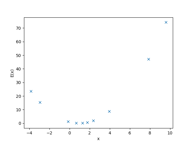
Fig. 39 Values of the objective function, \(\text{E}(x) = (1-x)^2\), versus random values of \(x\) selected by a simple random sampler.

Simple Workflow Example

This example uses the Ocean software package, dimod, to formulate a small objective function: the combinations() function generates a BQM that represents the problem of selecting exactly \(k\) of \(n\) binary variables.

The following code creates a BQM that is minimized when exactly two (\(k=2\)) of the three (\(n=3\)) variables a, b, c are \(1\):

>>> import dimod
>>> bqm = dimod.generators.combinations(['a', 'b', 'c'], 2)

Now solve on a D-Wave quantum computer using the DWaveSampler sampler from Ocean software’s dwave-system package. Also use its EmbeddingComposite composite to map the unstructured problem (variables such as \(a\) etc.) to the sampler’s graph structure (the QPU’s numerically indexed qubits) in a process known as minor-embedding.

The next code sets up a D-Wave quantum computer as the sampler.

Note

The following code sets a sampler without specifying SAPI parameters. Configure a default solver, as described in the Configuring Access to the Leap Service (Basic) section, to run the code as is, or see the dwave-cloud-client tool on how to access a particular solver by setting explicit parameters in your code or environment variables.

>>> from dwave.system import DWaveSampler, EmbeddingComposite
>>> sampler = EmbeddingComposite(DWaveSampler())

Because the sampled solution is probabilistic, returned solutions may differ between runs. Typically, when submitting a problem to the system, you ask for many samples, not just one. This way, you see multiple “best” answers and reduce the probability of settling on a suboptimal answer. Below, ask for 1000 samples.

>>> sampleset = sampler.sample(bqm, num_reads=1000, label='SDK Examples - QPU Workflow')
>>> print(sampleset)        
   a  b  c energy num_oc. chain_.
0  1  1  0    0.0     323     0.0
1  1  0  1    0.0     339     0.0
2  0  1  1    0.0     336     0.0
3  1  1  1    1.0       1     0.0
4  1  0  0    1.0       1     0.0
['BINARY', 5 rows, 1000 samples, 3 variables]

Almost all the returned samples represent valid value assignments for the \(\binom{N}{k}\) problem, and minima (low-energy states) of the BQM, and with high likelihood the best (lowest-energy: here \(0.0\) in the energy column) samples satisfy the formulation (two \(1\)s among the three variables columns, a, b, c).