

Penalty Models#
Penalty models represent constraints as small models, such as binary quadratic models (BQM), that have higher values for infeasible states (values of variables that violate the constraint). By adding such models to the objective function that represents your problem, you make it less likely that solutions that violate the constraint are selected by solvers that seek low-energy states.
Descriptive Example#
For example, consider that you are looking for solutions to a problem that is
represented by a binary quadratic model, bqm_p, which has variables
\(v_1, v_2, v_3, v_4, v_5, ...\) etc. You wish to constrain the solutions to
ones where \(v_2 \Leftrightarrow \neg v_4\); that is, variables \(v_2\)
and \(v_4\) never have the same value in good solutions.
The relation \(v_2 \Leftrightarrow \neg v_4\) represents a NOT gate, where one variable, say \(v_2\) is the gate’s input and the other, say \(v_4\) its output.
You can represent such a constraint with the penalty function:
This penalty function represents the constraint in that for assignments of
variables that match valid states (\(v_2 \ne v_4\)), the function evaluates
at a lower value than assignments that violate the constraint. Therefore, when
you minimize the sum of your objective function (bqm_p) and a BQM
representing this penalty function, those assignments of variables that meet the
constraint have lower values.
The table below shows that this function penalizes states that violate the constraint while no penalty is applied to assignments of variables that meet the constraint. In this table, columns \(\mathbf{v_2}\) and \(\mathbf{v_4}\) show all possible states of variables \(v_2\) and \(v4\); column Valid? shows whether the variables represent meet the constraint; column \(\mathbf{P}\) shows the value of the penalty for all possible assignments of variables.
\(\mathbf{v_2}\) |
\(\mathbf{v_4}\) |
Valid? |
\(\mathbf{P}\) |
|---|---|---|---|
\(0\) |
\(1\) |
Yes |
\(0\) |
\(1\) |
\(0\) |
Yes |
\(0\) |
\(0\) |
\(0\) |
No |
\(1\) |
\(1\) |
\(1\) |
No |
\(1\) |
For example, the state \(v_2, v_4 = 0,1\) of the first row represents valid assignments, and the value of \(P\) is
not penalizing the valid assignment of variables. In contrast, the state \(v_2, v_4 = 0,0\) of the third row represents an infeasible assignment, and the value of \(P\) is
adding a value of \(1\) to the BQM being minimized, bqm_p. By
penalizing both possible assignments of variables that violate the constraint,
the BQM based on this penalty function has minimal values (lowest energy states)
for variable values that meet the constraint.
Code Example#
Consider an example of mapping an AND clause to a QUBO. To do this,
solutions to the QUBO (solutions that minimize the energy of the QUBO) must be
exactly the valid configurations of an AND gate, z = AND(x_1, x_2).
First, import the required packages.
import penaltymodel as pm
import dimod
import networkx as nx
Next, determine the feasible configurations that the QUBO should target by minimizing the energy of these configurations. Below is a truth table representing an AND clause.
|
|
|
|---|---|---|
0 |
0 |
0 |
0 |
1 |
0 |
1 |
0 |
0 |
1 |
1 |
1 |
The rows of the truth table are exactly the feasible configurations.
feasible_configurations = [{'x1': 0, 'x2': 0, 'z': 0},
                           {'x1': 1, 'x2': 0, 'z': 0},
                           {'x1': 0, 'x2': 1, 'z': 0},
                           {'x1': 1, 'x2': 1, 'z': 1}]
At this point, you can get a penalty model.
bqm, gap = pm.get_penalty_model(feasible_configurations)
However, if you know the QUBO, you can build the penalty model yourself. Observe that for the equation,
E(x_1, x_2, z) = x_1 x_2 - 2(x_1 + x_2) z + 3 z + 0
you get the following energies for each row in the truth table:
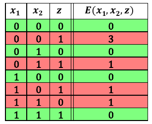
Fig. 249 Truth table for AND.#
The energy is minimized on exactly the desired feasible configurations; you can encode this energy function as a QUBO. Set the offset to zero because there is no constant energy offset.
qubo = dimod.BinaryQuadraticModel({'x1': 0., 'x2': 0., 'z': 3.},
                                  {('x1', 'x2'): 1., ('x1', 'z'): 2., ('x2', 'z'): 2.},
                                  0.0,
                                  dimod.BINARY)
The table shows a ground energy of 0; you can calculate it using the qubo to
check that this is true for the feasible configuration (0, 1, 0).
ground_energy = qubo.energy({'x1': 0, 'x2': 1, 'z': 0})
The last value needed is the classical gap. This is the difference in energy between the lowest infeasible state and the ground state.
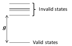
Fig. 250 Energy gap.#
With all of the pieces, you can now build the penalty model.
classical_gap = 1
p_model = pm.PenaltyModel.from_specification(spec, qubo, classical_gap, ground_energy)