Minor-Embedding: Best Practices

The D-Wave QPU minimizes the energy of an Ising spin configuration whose pairwise interactions lie on the edges of a QPU working graph, such as the Pegasus graph of an Advantage system. To solve an Ising spin problem with arbitrary pairwise interaction structure, the corresponding graph must be minor-embedded into a QPU’s graph.

There are algorithms that can embed a problem of \(N\) variables in at most \(N^2\) qubits.

Ocean software’s minorminer provides embedding tools.

Inspecting Minor-Embeddings

The dwave-inspector tool provides a graphic interface for examining D-Wave quantum computers’ problems and answers. As described in the Ocean workflow section, the D-Wave quantum computer solves problems formulated as binary quadratic models (BQM) that are mapped to its qubits in a process called minor-embedding. Because the way you choose to minor-embed a problem (the mapping and related parameters) affects solution quality, it can be helpful to see it.

For example, minor-embedding a problem represented by a \(K_5\) fully-connected graph into an Advantage quantum processing unit (QPU), with its Pegasus topology, requires representing one of the five variables with a chain of two physical qubits:

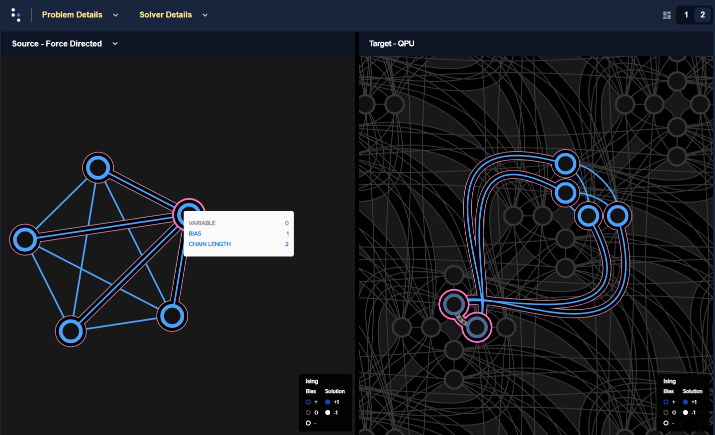
Fig. 147 Five-variable \(K_5\) fully-connected problem, shown on the left as a graph, is embedded in six qubits on an Advantage, shown on the right against the Pegasus topology. Variable 0, highlighted in dark magenta, is represented by two qubits, 1975 and 4840 in this particular embedding.

The problem inspector shows you your chains at a glance: you see lengths, any breakages, and physical layout.

Import the problem inspector to enable it[1] to hook into your problem submissions.

[1]

Importing the problem inspector activates for the session the capture of data such as problems sent to the QPU and returned responses, relevant details of minor-embedding, and warnings. The recommended workflow is to import it at the start of your coding session as is typical for Python packages (it is also possible, but less convenient, to specify in the submission that data such as embedding be returned with the response).

The following examples demonstrate the use of the show() method to visualize an embedded problem and a logical problem in your default browser.

Inspecting an Embedded Problem

This example shows the canonical usage: samples representing physical qubits on a QPU.

>>> from dwave.system import DWaveSampler
>>> import dwave.inspector
...
>>> # Get solver
>>> sampler = DWaveSampler(solver=dict(topology__type='pegasus'))
...
>>> # Define a problem (actual qubits depend on the selected QPU's working graph)
>>> h = {}
>>> J = {(2136, 4181): -1, (2136, 2151): -0.5, (2151, 4196): 0.5, (4181, 4196): 1}
>>> all(edge in sampler.edgelist for edge in J)     
True
>>> # Sample
>>> response = sampler.sample_ising(h, J, num_reads=100)    
...
>>> # Inspect
>>> dwave.inspector.show(response)   

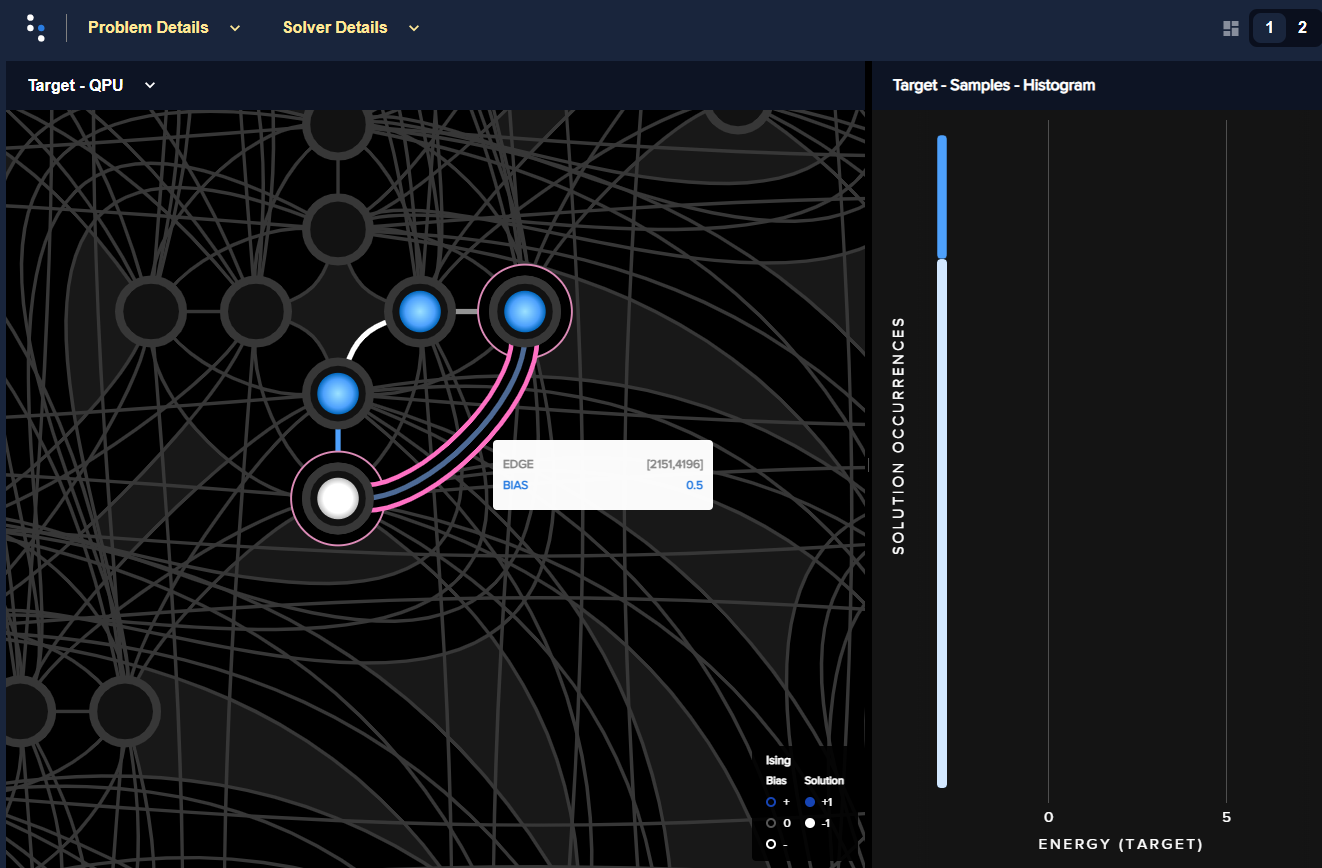
Fig. 148 Edge values between qubits 2136, 4181, 2151, and 4196, and the selected solution, are shown by color on the left; a histogram, on the right, shows the energies of returned samples.

Inspecting a Logical Problem

This example visualizes a problem specified logically and then automatically minor-embedded by Ocean’s EmbeddingComposite class. For illustrative purposes it sets a weak[2] chain_strength to show broken chains.

Define a problem and sample it for solutions:

>>> from dwave.system import DWaveSampler, EmbeddingComposite
>>> import dimod
>>> import dwave.inspector
...
>>> # Define problem
>>> bqm = dimod.generators.doped(1, 5)
>>> bqm.add_linear_from({v: 1 for v in bqm.variables})
...
>>> # Get sampler
>>> sampler = EmbeddingComposite(DWaveSampler())
...
>>> # Sample with low chain strength
>>> sampleset = sampler.sample(bqm, num_reads=1000, chain_strength=1)
...
>>> # Inspect the problem::
>>> dwave.inspector.show(sampleset)     

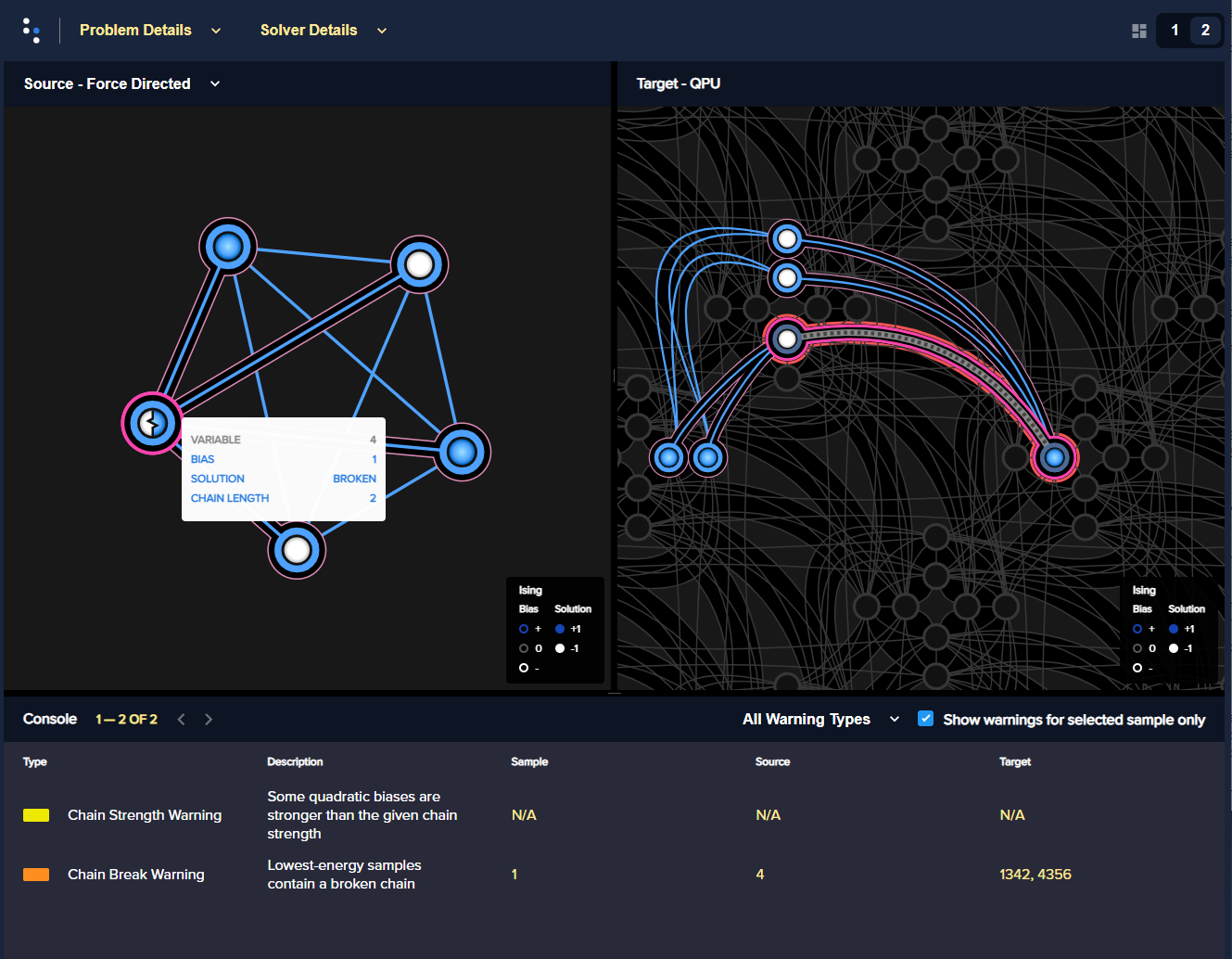
Fig. 149 The logical problem, on the left, shows that the value for variable 4 is based on a broken chain; the embedded problem, on the right, highlights the broken chain (its two qubits have different values) in bold red.

[2]

The default chain strength was about 3 for similar problems.

Global Versus Local

Global embedding models each constraint as a BQM, adds all constraint models, and maps the aggregate onto the QPU graph. Advantages of this method are that it typically requires fewer qubits and shorter minor embedding.

Locally structured embedding models each constraint locally within a subgraph, places the local subgraphs within the QPU graph, and then connects variables belonging to multiple local subgraphs. Advantages of this method, when the scopes of constraints are small, are typically that it is more scalable to large problems, requires less precision for parameters, and enforces qubit chains with lower coupling strengths.

Example

The two graphics below compare local and global embeddings onto an Advantage QPU of a BQM represented by a graph composed of three \(K_5\) cliques (fully connected five-node graphs), sparsely interconnected.

• Figure 150 shows a local embedding: each \(K_5\) subgraph is manually embedded using the FixedEmbeddingComposite class into a \(K_{4,4}\)-like structure of the Pegasus graph.

• Figure 151 shows a global embedding: the entire BQM is embedded using the EmbeddingComposite class.

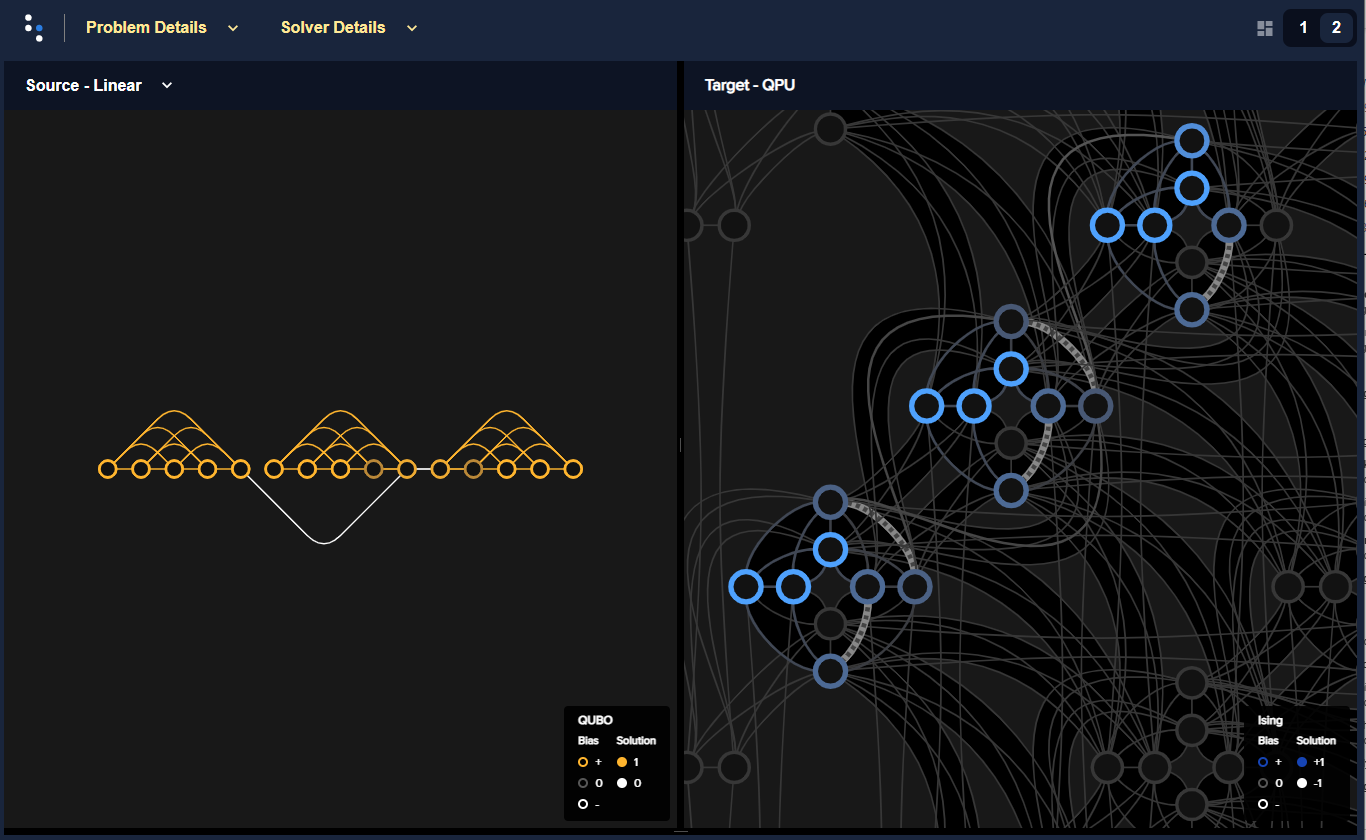
Fig. 150 Example of local embedding for a BQM represented by a graph of three connected \(K_5\) cliques.

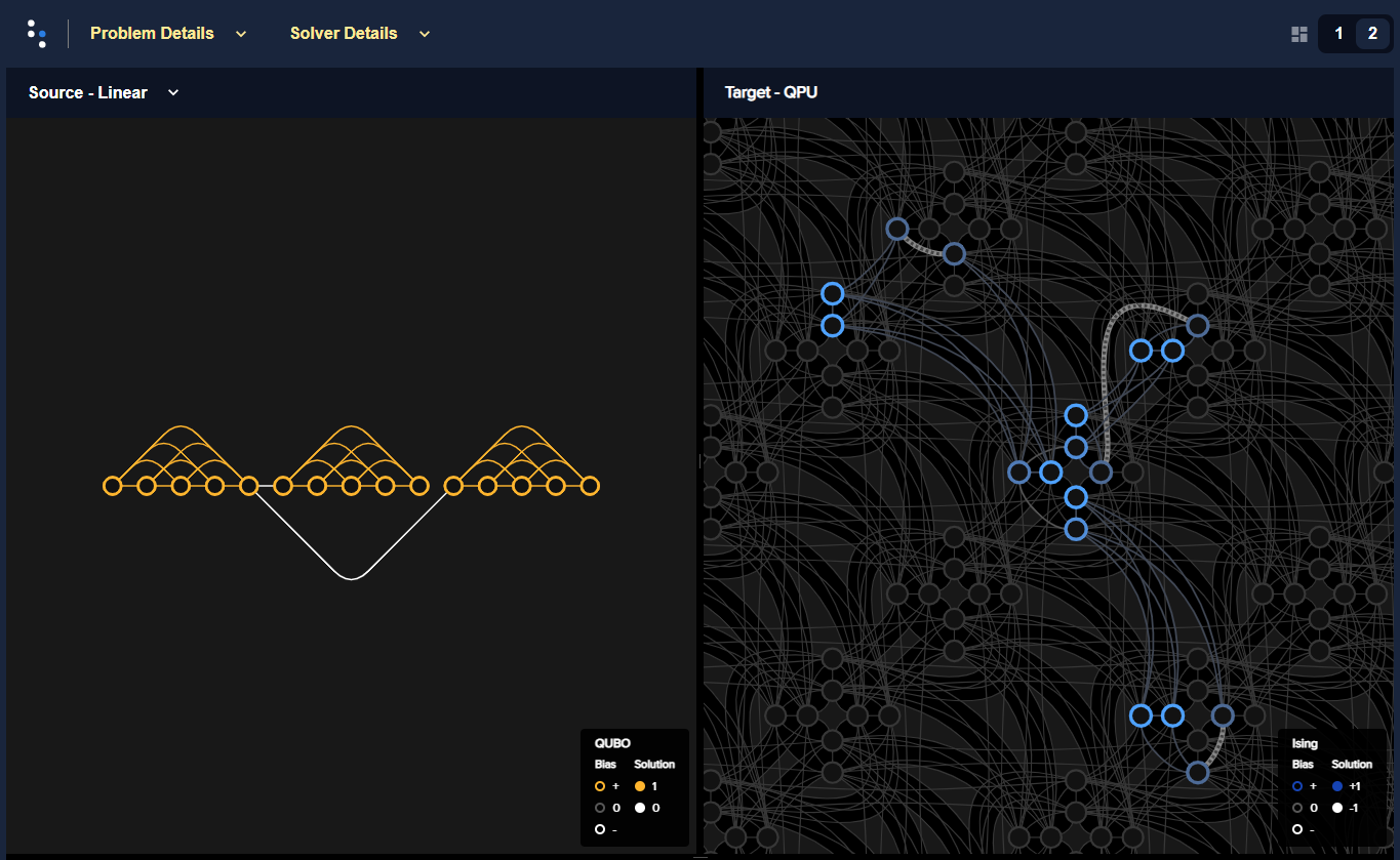
Fig. 151 Example of global embedding for a BQM represented by a graph of three connected \(K_5\) cliques.

In this small example, global embedding is likely more performant but for a larger number of repeated subgraphs, local emebedding with its repeated structure likely would keep chains shorter and uniform across the entire problem (assuming simple and sparse connectivity between parts).

Further Information

• [Bia2016] compares global and local methods of embedding in the context of CSPs and discusses a rip-up and replace method.

• [Boo2016] discusses clique minor generation.

• [Cai2014] gives a practical heuristic for finding graph minors.

• [Jue2016] discusses using FPGA-like routing to embed.

• [Ret2017] describes embedding quantum-dot cellular automata networks.

Chain Management

Similar to Lagrangian relaxation, you map a given problem’s variable \(s_i\) onto chain \(\{q_i^{(1)}, \cdots, q_i^{(k)}\}\) while encoding equality constraint \(q_i^{(j)} = q_i^{(j')}\) as an Ising penalty \(-M q_i^{(j)} q_i^{(j')}\) of weight \(M > 0\).

The following considerations and recommendations apply to chains.

• Prefer short chains to long chains.

• Prefer uniform chain lengths to uneven chains.

• Balance chain strength and problem range. Estimate chain strength and set just slightly above the minimum threshold needed, using strategies for auto-adjusting these chains. When mapping a problem’s variable to qubits chains, the penalties for equality constraints should be (1) large enough so low-energy configurations do not violate these constraints and (2) the smallest weight that enforces the constraints while enabling precise problem statement (on \(\vc{h}\) and \(\vc{J}\)) and efficient exploration of the search space. An effective procedure incrementally updates weights until the equality constraints are satisfied.

  See also the Imprecision of Biases section.

Example

This example embeds a BQM representing a 30-node signed-social network problem and then looks at the effects of different chain-strength settings.

>>> import networkx as nx
>>> import random
>>> import numpy as np
>>> import dwave_networkx as dnx
>>> import dimod
>>> from dwave.system import DWaveSampler, LazyFixedEmbeddingComposite
>>> import dwave.inspector
...
>>> # Create a problem
>>> G = nx.generators.complete_graph(30)
>>> G.add_edges_from([(u, v, {'sign': 2*random.randint(0, 1) - 1}) for u, v in G.edges])
>>> h, J = dnx.algorithms.social.structural_imbalance_ising(G)
>>> bqm = dimod.BQM.from_ising(h, J)
>>> # Sample on a D-Wave system
>>> num_samples = 1000
>>> sampler = LazyFixedEmbeddingComposite(DWaveSampler())
>>> sampleset = sampler.sample(bqm, num_reads=num_samples)      

You can now analyze the solution looking for the affects of your chain-strength setting in various ways.

As a first iteration, it’s convenient to use the Ocean software’s default chain strength. The LazyFixedEmbeddingComposite class sets a default chain strength using the uniform_torque_compensation() function to calculate a reasonable value. For this problem, with the embedding found heuristically, it calculated a chain strength of about 7.

>>> print(sampleset.info["embedding_context"]["chain_strength"]) 
7.614623037288188

You can check the length of the longest chain.

>>> chains = sampleset.info["embedding_context"]["embedding"].values()  
>>> print(max(len(chain) for chain in chains))               
6

You can verify that the default chain strength for this problem is strong enough so few chains are broken.

>>> print("Percentage of samples with >10% breaks is {} and >0 is {}.".format(
...       np.count_nonzero(sampleset.record.chain_break_fraction > 0.10)/num_samples*100,
...       np.count_nonzero(sampleset.record.chain_break_fraction > 0.0)/num_samples*100)) 
Percentage of samples with >10% breaks is 0.0 and >0 is 17.5.

You can also look at the embedding and histograms of solution energies using the Ocean software’s problem inspector tool.

>>> dwave.inspector.show(sampleset)                       

Figure 152 shows the BQM embedded in an Advantage QPU.

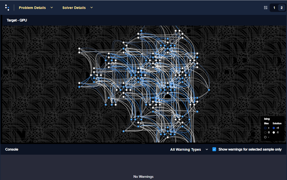
Fig. 152 BQM representing a social-network problem of 30 nodes embedded in an Advantage QPU.

The following graphs show histograms of the returned solutions’ energies for different chains strengths:

• Figure 153 has the default chain strength, which for this problem was calculated as about 7.

• Figure 154 has a chain strength manually set to 1 (identical to the maximum bias for the problem). [3]

• Figure 155 has a chain strength manually set to 14 (double the default value for this problem).

[3]

You can set a chain strength relative to your problem’s largest bias by using, for example, the scaled() function.

>>> from dwave.embedding.chain_strength import scaled
...
>>> sampleset = sampler.sample(
...     bqm, num_reads=num_samples, chain_strength=scaled)  

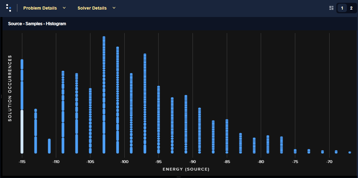
Fig. 153 Energy histogram for the social-network problem with a chain strength of ~7.

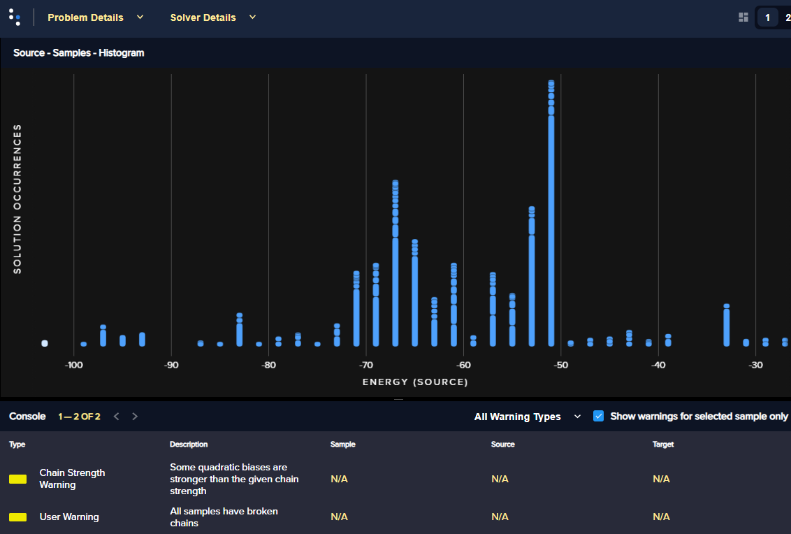
Fig. 154 Energy histogram for the social-network problem with a chain strength of 1.

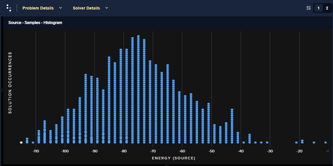
Fig. 155 Energy histogram for the social-network problem with a chain strength of 14.

You can see that setting the chain strength too low compared to the problem’s biases results in high chain breakage and consequently few good solutions; setting it too high distorts the problem.

Further Information

• The Multiple-Gate Circuit example is a good introductory example of the effects of setting chain strengths.

• The Using the Problem Inspector example demonstrates using the Ocean software’s problem inspector tool for examining embeddings and setting chain strengths.

• [Rie2014] studies embedding and parameter setting, and their effects on problem solving in the context of optimization problems.

• [Ven2015b] discusses effects of embedding the Sherrington-Kirkpatrick problem.

Embedding Complete Graphs

Embeddings for cliques (fully-connected graphs) can be very useful: a minor-embedding for a \(K_n\) clique can be used for all minors of that graph. This means that if your application needs to submit to the QPU a series of problems of up to \(n\) variables, having an embedding for the \(K_n\) graph lets you simply reuse it for all those submissions, saving the embedding-computation time in your application’s runtime execution.

Using a clique embedding can have a high cost for sparse graphs because chain lengths increase significantly for high numbers of variables.

Example: Largest Cliques on the Chimera Topology

The largest complete graph \(K_V\) that is a minor of a \(M\times N\times L\) Chimera graph has \(V=1+L\min(M,N)\) vertices. For example, 65 vertices is the theoretical maximum on a C16 Chimera graph (a \(16 {\rm x} 16\) matrix of 8-qubit unit cells for up to[4] \(2MNL=2 \times 16 \times 16 \times 4=2048\) qubits), which was the topology of the D-Wave 2000Q system.

[4]

The yield of a working graph is typically less than 100%.

Example: Chain Lengths for Cliques on Pegasus and Chimera Topologies

Table 52 shows some example embeddings of complete graphs versus chain lengths for both QPU topologies with 95% yields. For a given maximum chain length, you can embed cliques of about the following sizes in Pegasus P16 and Chimera C16 topologies with working graphs simulating 95% yield (by random removal of 5% of nodes and 0.5% of edges to represent inactivated qubits and couplers):

Table 52 Complete Embeddings Versus Chain Length for 95% Yields.

Chain Length	Chimera Topology	Pegasus Topology
1	\(K_2\)	\(K_4\)
2	\(K_4\)	\(K_{10}\)
4	\(K_{12}\)	\(K_{30}\)
10	\(K_{28}\)	\(K_{71}\)

For a Pegasus graph with 100% yield the largest complete graph that is embeddable is \(K_{150}\) with chain length of 14. QPUs typically do not achieve 100% yield.

Example: Clique-Embedding a Sparse BQM

Figure 156 shows an example BQM constructed from a sparse NetworkX graph, chvatal_graph(). This example embeds the BQM onto an Advantage QPU in two ways: (1) using the standard minorminer heuristic of the EmbeddingComposite class and (2) using a clique embedding found by the DWaveCliqueSampler class.

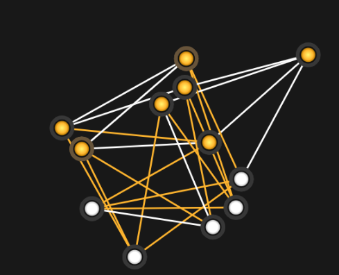
Fig. 156 BQM based on a sparse graph.

>>> from dwave.system import DWaveSampler, EmbeddingComposite, DWaveCliqueSampler
>>> import networkx as nx
>>> import dimod
>>> import random
>>> import dwave.inspector
...
>>> # Create a small, sparse BQM from a NetworkX graph
>>> G = nx.generators.small.chvatal_graph()
>>> for edge in G.edges:
...     G.edges[edge]['quadratic'] = random.choice([1,-1])
>>> bqm = dimod.from_networkx_graph(G,
...                                 vartype='BINARY',
...                                 edge_attribute_name='quadratic')
>>> sampleset = EmbeddingComposite(DWaveSampler()).sample(bqm, num_reads=1000)
>>> sampleset_clique = DWaveCliqueSampler().sample(bqm,
...                                                num_reads=1000) 

The following graphs show both embeddings:

• Figure 157 is an embedding found for the sparse graph.

• Figure 158 is a clique embedding in which the BQM graph is a minor.

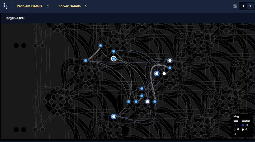
Fig. 157 Embedding found for the sparse graph of the problem.

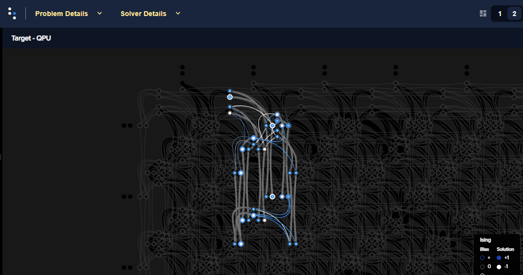
Fig. 158 Clique embedding that includes the sparse graph of the problem.

Clearly the clique embedding requires more and longer chains.

Further Information

• [Pel2021] proposes a method of parallel quantum annealing that makes use of available qubits by embedding several small problems in the same annealing cycle.

• [Zbi2020] proposes two algorithms, Spring-Based MinorMiner (SPMM) and Clique-Based MinorMiner (CLMM), for minor-embedding QUBO problems into Chimera and Pegasus graphs.

• Exploring the Pegasus Topology Jupyter Notebook.

Reusing Embeddings

For problems that vary only the biases and weights on a fixed graph, you can set a good embedding once before submitting the problem to the QPU. There is no need to recompute the embedding (a time-consuming operation) for every submission.

Pre-embedding Local Constraint Structures

The structure of some problems contains repeated elements; for example, the multiple AND gates, half adders, and full adders in the Factoring example. Such problems may benefit from being embedded with repeating block structures for the common elements, with connectivity then added as needed.

Example

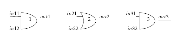
Fig. 159 Circuit of three Boolean gates.

This small example pre-embeds three Boolean gates.

You can embed a BQM representing an AND or OR gate in a repeating structure of the Pegasus topology, a \(K_{4,4}\) biclique with additional couplers connecting some horizontal and vertical qubits.

>>> import minorminer
>>> import dwave_networkx as dnx
>>> from dimod.generators import and_gate, or_gate
...
>>> pegasus_k44 = dnx.pegasus_graph(2, node_list=[4, 5, 6, 7, 40, 41, 42, 43])
...
>>> bqm_and1 = and_gate('in11', 'in12', 'out1')
>>> embedding_and = minorminer.find_embedding(list(bqm_and1.quadratic.keys()), pegasus_k44)
>>> embedding_and                                           
{'in12': [40], 'in11': [4], 'out1': [41]}
...
>>> bqm_or2 = or_gate('in21', 'in22', 'out2')
>>> embedding_or = minorminer.find_embedding(list(bqm_or2.quadratic.keys()), pegasus_k44)
>>> embedding_or                                        
{'in22': [4], 'in21': [41], 'out2': [40]}

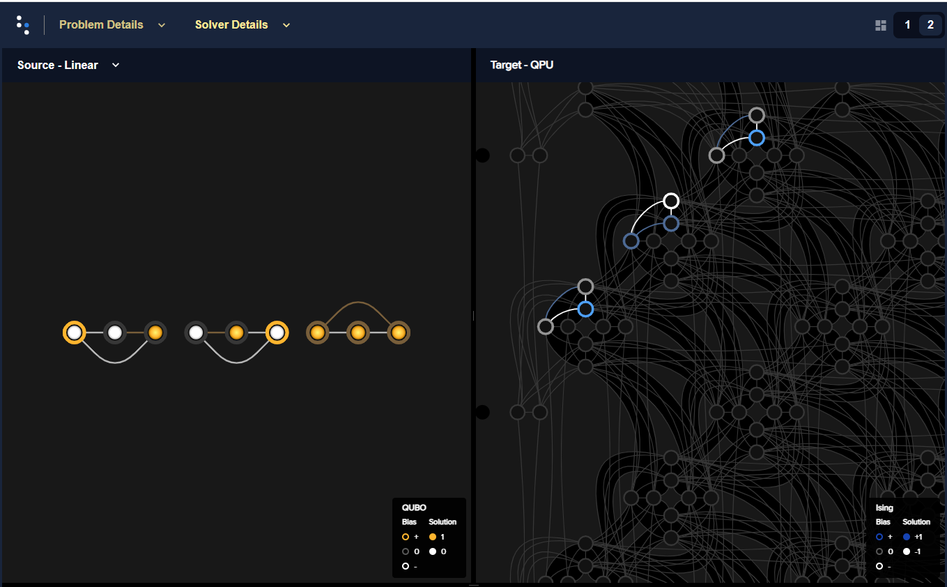
Fig. 160 Circuit of three Boolean gates pre-embedded in an Advantage QPU.

Further Information

• [Ada2015] describes embedding an RBM on the D-Wave system by mapping the visible nodes to chains of vertical qubits and hidden nodes to chains of horizontal qubits.

Virtual Graphs

Important

The virtual graph feature is deprecated due to improved calibration of newer QPUs: Ocean software’s VirtualGraphComposite class will be removed in a future release. To calibrate chains for residual biases, follow the instructions in [Che2023].

The D-Wave virtual graph feature simplifies the process of minor-embedding by enabling you to more easily create, optimize, use, and reuse an embedding for a given working graph. When you submit an embedding and specify a chain strength using the VirtualGraphComposite class, it automatically calibrates the qubits in a chain to compensate for the effects of unintended biases—see integrated control errors (ICE) 1—caused by QPU imperfections.

Further Information

• [Dwave6] is a white paper describing measured performance improvements from using virtual graphs.