Errors and Error Correction

This section presents the following topics.

• ICE describes integrated control errors (ICE) as a source of errors.

• Other Error Sources describes additional sources of errors.

• Error-Correction Features describes measures to correct these errors.

ICE

The dynamic range of \(h\) and \(J\) values may be limited by integrated control errors (ICE). The term ICE refers collectively to these sources of infidelity in problem representation. This chapter provides an overview of ICE, describes the main sources that contribute to it, and provides guidance on measuring its effects.

Note

Data given in this chapter are representative of D-Wave systems.

Overview of ICE

Although \(h\) and \(J\) may be specified as double-precision floats, some loss of fidelity occurs in implementing these values in the D-Wave QPU. This fidelity loss may affect performance for some types of problems.

Specifically, instead of finding low-energy states to an optimization problem defined by \(h\) and \(J\) as in equation qpu_equation_ising_objective, the QPU solves a slightly altered problem that can be modeled as

\begin{equation} E^{\delta}_{ising} ({\bf s}) = \sum_{i=1}^N (h_i + \delta h_i ) s_i + \sum_{i=1}^N \sum_{j=i+1}^{N} (J_{i,j} + \delta J_{i,j} ) s_i s_j, \end{equation}

where \(\delta h_i\) and \(\delta J_{i,j}\) characterize the errors in parameters \(h_i\) and \(J_{i,j}\), respectively.[1]

[1]

Because \(\delta h\) and \(\delta J\) are summed over \(N\), fidelity limitations tend to have a greater effect on performance for full-QPU sized problems, for a given dynamic range and distribution of \(h\) and \(J\).

The error \(\delta h_i\) depends on \(h_i\) and on the values of all incident couplers \(J_{i,j}\) and neighbors \(h_j\), as well as their incident couplers \(J_{j,k}\) and next neighbors \(h_k\). That is, if spin \(i\) is connected to spin \(j\), and spin \(j\) is connected to spin \(k\) in the topological graph, then \(\delta h_i\) may depend, to varying extents, on \(h_i, h_j, h_k\), \(J_{i,j}\), and \(J_{j,k}\). This dependency holds when the relevant qubits and couplings are present in the graph, irrespective of whether they are set to nonzero values. Similarly, \(\delta J_{i,j}\) depends on spins and couplings in the local neighborhood of \(J_{i,j}\). For example, if a given problem is specified by \((h_1 = 1 , h_2 = 1, J_{1,2} = -1)\), the QPU might actually solve the problem \((h_1 = 1.01, h_2 = 0.99, J_{1,2} = -1.01)\). Changing just a single parameter in the problem could change all three error terms, altering the problem in different ways.

The probability distribution of \(\delta h\) and \(\delta J\) is an ensemble across a set of problem settings \(h\) and \(J\) and across all \(i\) and \(i,j\) pairs. The \(\delta h\) and \(\delta J\) values are Gaussian-distributed with mean \(\mu\) and standard deviation \(\sigma\) that vary with anneal fraction \(s\) during the anneal.[2] The QPU control system is calibrated so that there is typically a value of \(s\) for which \(\mu\) is zero. This point is chosen to be somewhere between the single qubit freezeout point described in the Freezeout Points section (later in the anneal), and at the quantum critical point of a one-dimensional Ising chain (earlier in the anneal). Distributions with nonzero \(\mu\) for some values of \(s\) are considered to be due to systematic errors discussed later in this chapter. Thus, the expected deviations of \(h\) and \(J\) during operation are the sum of a systematic contribution \(\mu\) and a random component with standard deviation \(\sigma.\)

[2]

Assumed for simplicity; distributions seen in actual results are close to this.

Figure 120 and Figure 121 show example measurements of \(\delta h\) and \(\delta J\) distributions at different fractional times \(s\). See the Using Two-Spin Systems to Measure ICE section for a description of the measurement method.

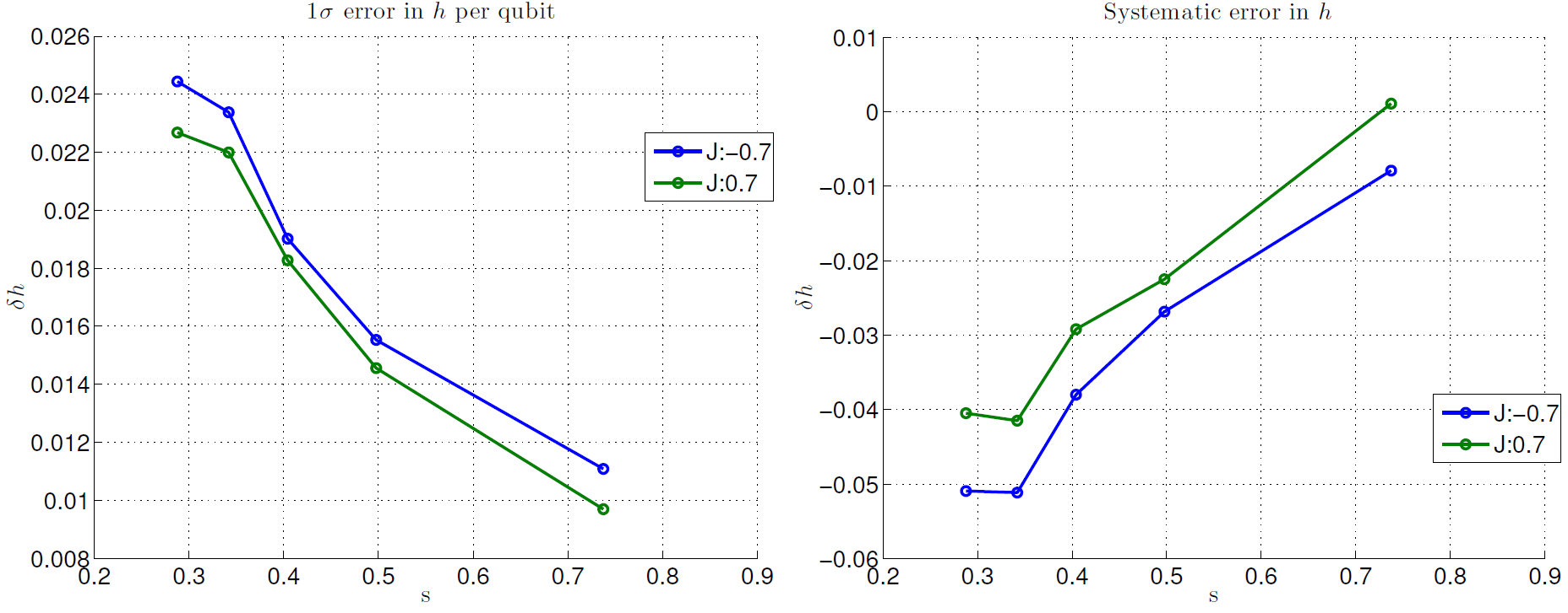
Fig. 120 \(\delta h\) distributions estimated from best-fit parameters to a thermal model. The left plot shows the standard deviation of the distribution and the right plot shows the mean. Data were taken for logical qubits between size 1 (larger \(s\)) and size 5 (smaller \(s\)) to get an estimate of \(\delta h\) over a range of \(s\). Data shown are representative of D-Wave 2X systems.

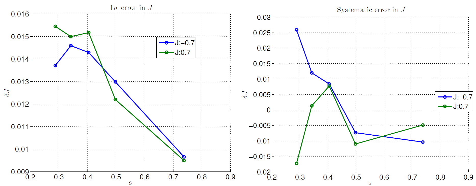
Fig. 121 \(\delta J\) distributions estimated from best-fit parameters to a thermal model. The left plot shows the standard deviation of the distribution and the right plot shows the mean. Data were taken for logical qubits between size 1 (larger \(s\)) and size 5 (smaller \(s\)) to get an estimate of \(\delta J\) over a range of \(s\). Data shown are representative of D-Wave 2X systems.

Sources of ICE

The Ising spins on the D-Wave QPU are intrinsically analog, controlled through spatially local magnetic fields. The controls are a combination of the output of DACs and other analog signals shared among groups of spins. A calibration procedure, conducted when the QPU first comes online, determines the mapping between Ising problem specifications \(h\) and \(J\), and the control values used during annealing.

QPU calibration is a significant part of the time required to install a D-Wave system at a site. It involves a series of measurements of the QPU and the refrigerator to obtain data used to build models that achieve the desired Ising spin Hamiltonian.

These models identify several factors that contribute to distortions of \(h\) and \(J\) due to ICE. Understanding these factors, and how to compensate for them, can guide your choices in \(h\) and \(J\) when you specify a problem. Listed below are the dominant sources of ICE. The subsections that follow give additional details.

• Background Susceptibility (ICE1)

  The qubits behave weakly as couplers, which leads to effective next-nearest-neighbor (NNN) \(J\) interactions and a leakage of applied \(h\) biases from a qubit to its neighbors.

• Flux Noise of the Qubits (ICE2)

  The qubits experience low-frequency \(1/f\)-like flux noise. This noise contributes an error that varies in time (that is, between runs on the QPU), and also varies with \(s\).

• DAC Quantization (ICE3)

  The DACs that provide the specified \(h\) and \(J\) values have a finite quantization step size.

• I/O System Effects (ICE4)

  The ratio of \(h/J\) may differ slightly for different annealing parameters such as \(t_f\).

• Distribution of h Scale Across Qubits (ICE5)

  Qubits cannot be made perfectly identical. As a result, individual spins may have slightly different magnitudes (persistent currents) and tunneling energies. These differences also vary with anneal fraction \(s\).

Background Susceptibility

During the annealing process, every Ising spin has a coupler-like effect on its neighbors (that is, the spins to which it is connected by couplings) that is not captured by the problem Hamiltonian. This effect takes two main forms:

• Spin \(i\) induces next-nearest neighbor (NNN) couplings between pairs of its neighboring spins.

• The applied \(h\) bias leaks from spin \(i\) to its neighboring spins.[3]

[3]

A more detailed description of how this arises from flux qubits is in [Har2010].

The strength of this background susceptibility effect is characterized by a parameter \(\chi\).[4]

[4]

Use of the \(\chi\) symbol is consistent with the usage in physics of \(\chi\) to characterize the susceptibility of a magnetic system. This document uses a normalized \(\chi = M_{\rm AFM} \chi_q\), where \(M_{\rm AFM}\) is the maximum available antiferromagnetic mutual inductance, and \(\chi_q = \frac{dI_p}{d\Phi_q}\) is the physical qubit susceptibility.

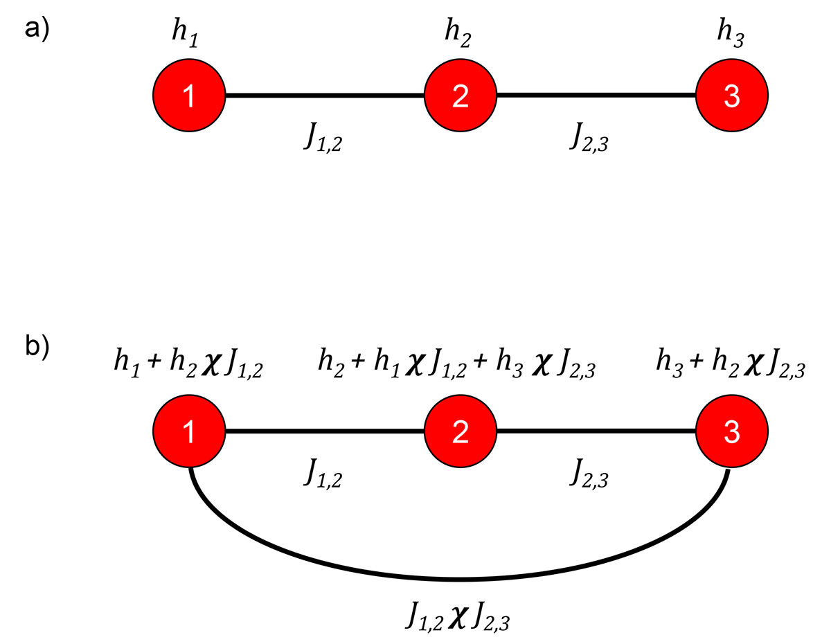
Fig. 122 a) Three-spin system to look at the effect of \(\chi\). Three spins, red circles, labeled \(1, 2, 3\) with local \(h\)-biases of \(h_1, h_2, h_3\), respectively, and couplings between neighboring spins denoted by lines of \(J_{1,2}\) between spin \(1\) and spin \(2\), and \(J_{2,3}\) between spin \(2\) and spin \(3\). b) The model for the system showing induced couplings and \(h\)-biases due to qubit susceptibility, \(\chi\).

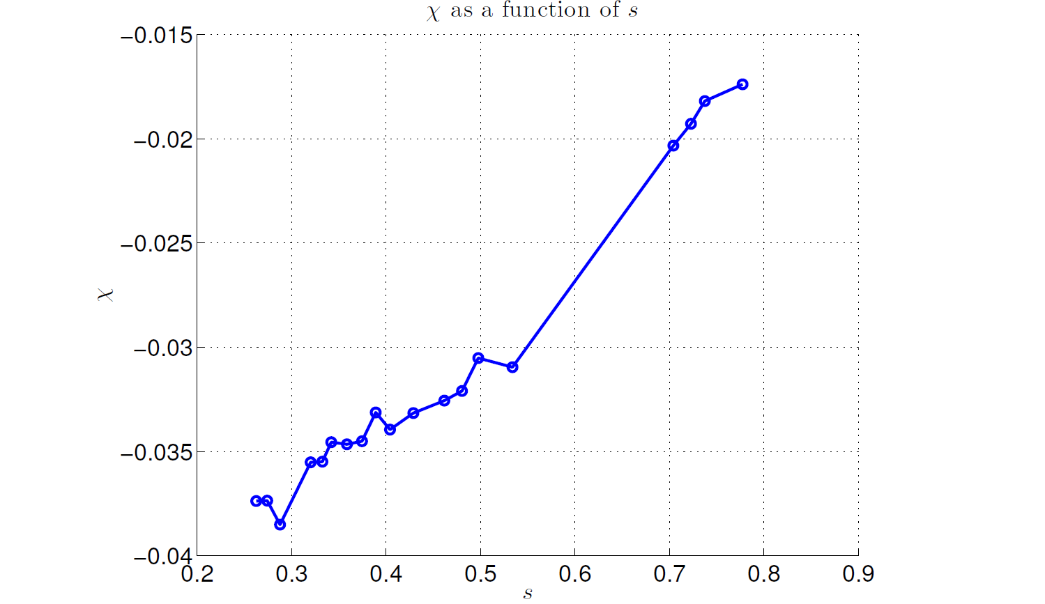
Fig. 123 \(\chi\) variation during the anneal. Data shown are representative of D-Wave 2X systems.

For example, consider the three-spin problem shown in Figure 122. This system is described by the Ising energy function

\begin{equation} E_{3} (\vc s) = + h_1 s_1 + h_2 s_2 + h_3 s_3 + J_{1,2} s_1 s_2 + J_{2,3} s_2 s_3. \end{equation}

The energy function solved by the QPU, however, has some extra terms:

\begin{equation} E^\delta_{\chi} (\vc s) = \underbrace{ + h_2 \chi J_{1,2} s_1 + h_1 \chi J_{1,2} s_2 + h_3 \chi J_{2,3} s_2 + h_2 \chi J_{2,3} s_3 }_\text{$h$ leakage} + \underbrace{ J_{1,2} \chi J_{2,3} s_1 s_3 }_\text{NNN coupling}. \end{equation}

The NNN coupling occurs because spin 1 induces an interaction between spins 1 and 3 with magnitude \(J_{1,2} \chi J_{2,3}\). Similarly, \(h_2\) leaks onto spin 1, with magnitude \(h_2 \chi J_{1,2}\), and so on for the other terms.

Figure 123 shows how \(\chi\) typically varies with \(s\), from around -0.04 early in the anneal to near -0.015 late in the anneal, at which point single-spin dynamics freeze out.

Flux Noise of the Qubits

As another component of ICE, each \(h_i\) is subject to an independent (but time-dependent) error term that comes from the \(1/f\) flux noise of the qubits.[5] There are fluctuations in the flux noise that have lower frequency than the typical inverse annealing time, so problems solved in quick succession have correlated contributions from flux noise. By default, flux drift is automatically corrected every hour by the D-Wave system so that it is bounded and approximately Gaussian when averaged across all times; see the Drift Correction section for the procedure. You can disable this automatic correction by setting the flux_drift_compensation solver parameter to False. If you do so, apply flux-bias offsets manually; see the Calibration Refinement section.

[5]

Couplers also have \(1/f\) flux noise, but this effect is insignificant compared to \(\delta h\) and \(\delta J\).

Because the physical source of noise is flux fluctuations on the qubits, the effective level of noise is larger earlier in the anneal when the persistent current in qubits is smaller, so that \(h\) is relatively smaller in physical flux units; see the Hardware: Coupled Flux Qubits section and the Characterizing the Effect of Flux Noise section for details.

The Fourier spectrum of the fluctuations of \(\delta h^2\) varies approximately as \(A^2/f^\alpha\), where \(f\) is frequency from 1 mHz to the highest-resolvable frequency, \(A\) is the amplitude of the fluctuations at \(f = 1\) Hz, and \(\alpha\) is the spectral tilt—or frequency dependence—of the fluctuations. Due to the flux drift compensation, the spectrum becomes flat and close to zero below 1 mHz. Integrating the noise from 1 mHz to 1 MHz (the relevant band of interest observable directly), the Gaussian contribution to \(\delta h\) is approximately 0.009 early in the anneal and less later in the anneal. Figure 124 shows typical data for a 64-qubit system.

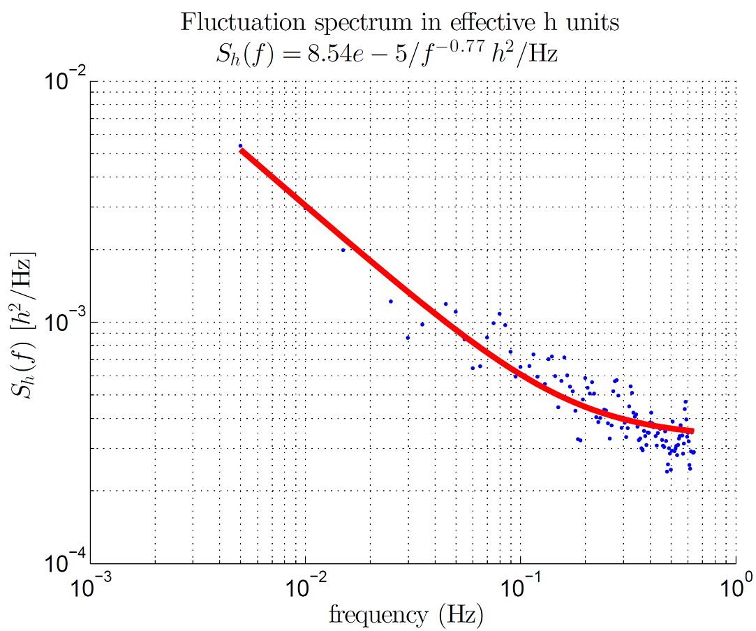
Fig. 124 Power spectral density of \(h\) fluctuations for a 64-qubit cluster. Data are taken by strongly coupling 64 qubits together and measuring the magnetization fluctuation of the system over time. The power spectral density of this signal, in effective \(h\) units, is plotted as a function of frequency. The solid line shows a best fit to the model \(A^2/f^{\alpha} + wn\), where \(wn\) is the statistical noise floor of the measurement technique and is not a measurement of any intrinsic broadband fluctuation of the qubit environment. See the Characterizing the Effect of Flux Noise section for more details. Data shown are representative of D-Wave 2X systems.

DAC Quantization

The DACs that provide the user-specified \(h\) and \(J\) values have a finite quantization step size. That step size depends on the value of the \(h\) or \(J\) applied because the response to the DAC output is nonlinear.

This random error contribution is described by a uniform distribution centered at 0 and having errors \(\pm b\). Typical errors for \(h\) and \(J\) are shown in Figure 125. Note that these errors are smaller than other contributors to ICE.

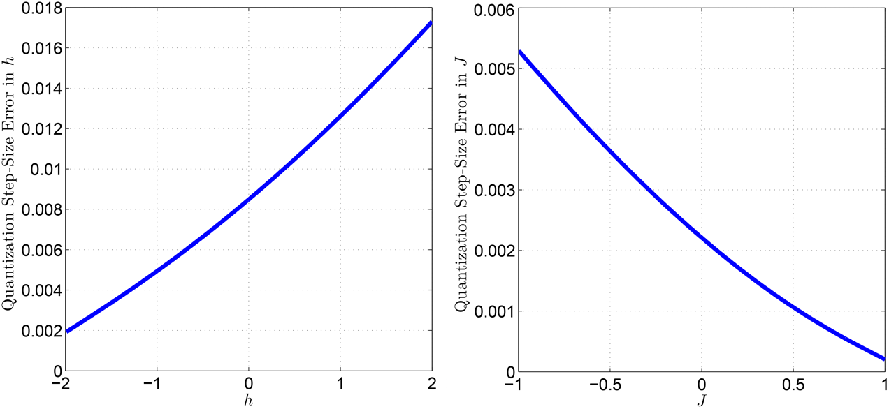
Fig. 125 Typical quantization step for the DAC controlling the \(h\) parameter (left) and \(J\) parameter (right). For example, \(h = 0.000\) may be off by as much as \(\pm 0.008\) when realized on the QPU. Over all qubits, you might find a worst-case qubit biased with \(h = 0.008\), and another worst-case qubit biased with \(h = -0.008\). Data shown are representative of D-Wave 2X systems.

I/O System Effects

Several time-dependent analog signals are applied to the QPU during the annealing process. Because the I/O system that delivers these signals has finite bandwidth,[6] the waveforms must be tuned for each anneal to minimize any potential distortion of the signals throughout the annealing process. As a result, the ratio of \(h/J\) may vary slightly with \(t_f\) and with scaled anneal fraction \(s\).

[6]

The anneal and h-controlling waveforms—\(\Phi_{\rm CCJJ}(s)\) and \(\Phi^x_i(s)\) terms, respectively, of equation (2) in the Annealing Implementation and Controls section—pass through low-pass filters with the following cutoff frequencies:

• For \(\Phi_{\rm CCJJ}(s)\): 30 MHz on both Advantage and Advantage2™ systems

• For \(\Phi^x_i(s)\): 3 MHz for Advantage systems and 30 MHz for Advantage2 systems

Distribution of \(h\) Scale Across Qubits

Assuming a fixed temperature of the system, and \(J=0\), the expected graph of the relationship between user-specified \(h\) and QPU-realized \(h\) has slope = 1, reflecting a constant mean offset \(\mu\) in the distribution of \(\delta h\). The measured slopes, however, are different for each spin, and are Gaussian-distributed.

This divergence results from small variations in the physical size of each qubit and from imperfections that arise when attempting to homogenize the macroscopic parameters—physical inductance \(L\), capacitance \(C\), and Josephson junction critical current \(I_c\)—across all physical qubits in the QPU.

Assuming a fixed temperature for the system, the ideal relationship, or slope, between qubit population and applied \(h\) is identical across an ensemble of devices. The distribution of measured slopes, however, is Gaussian-distributed with a standard deviation of approximately 1%, which contributes to \(\delta h\) and \(\delta J\). This distribution results from differences in the magnitude of each spin \(s_i\); see the Using Two-Spin Systems to Measure ICE section.

Measuring ICE

This section describes how to measure the effects of \(1/f\) noise as well as how to harness effective two-spin systems to measure the effects of ICE.

Measuring \(1/f\) Noise

A straightforward way to look at the \(1/f\) noise in the \(h\) parameter is to set all \(h\) and \(J\) values equal to 0 on the full QPU and observe how resulting qubit distributions drift over time in repeated tests. This approach identifies the effective \(1/f\) noise error on \(h\) when referenced to the single qubit freezeout point \(s^*_q\). To probe the \(1/f\) noise at earlier anneal times (and to amplify the error signal), create clusters of strongly coupled qubits and measure the time-dependent behavior of the net magnetization of system as described in the next section.

Using Two-Spin Systems to Measure ICE

You can use the results of problems defined on pairs of Ising spins scattered over the topological graph to help to characterize ICE effects.

Simple Two-Spin Systems

The simplest version of such problems has two Ising spins with biases \(h_1\) and \(h_2\) and a coupling between them of weight \(J\). The energy of this system is

(3)\[ E_{2spin}(\vc s) = +h_1 s_1 + h_2 s_2 + J s_1 s_2.\]

To measure ICE using simple two-spin systems, first find all independent edge sets of the available graph; that is, the sets of two-spin systems that can be manipulated independently. Simultaneously, for each set, ask the QPU to solve the independent two-spin problems at a variety of \(h_1\) and \(h_2\) settings near the phase boundaries indicated in Figure 126. Then fit the resulting data to a thermal model to estimate the deviations, \(\delta h\) and \(\delta J\), from equation (3) above using the correction terms of equation (4) below.

The two-spin phase diagram in Figure 126 characterizes the lowest energy state of the system as a function of \(h_1\) and \(h_2\) for given \(J\), here set to \(J=-0.5\). The dashed line delineates regions of the \(h_1\) and \(h_2\) space where resulting Ising spins are indicated by the up (\(s = 1\)) and down (\(s = -1\)) arrows. Applying a larger magnitude (more negative) \(J\) value increases ferromagnetic interactions, growing the regions of \(\downarrow \downarrow\) and \(\uparrow \uparrow\) while shrinking the regions of \(\downarrow \uparrow\) and \(\uparrow \downarrow\).

The ideal diagram may be compared to one obtained assuming the existence of background susceptibility errors. For this problem, the \(\chi\) correction terms are

(4)\[ E^\delta_{2spin} (\vc s) = +h_2 \chi J s_1 + h_1 \chi J s_2.\]

The \(h\)-leakage effects are shown in Figure 126: the blue lines denote the boundaries of the different spin ordering regions for the case where \(\chi = -0.05\), versus the ideal case shown by the dashed lines. (The two-spin system does not have NNN effects.)

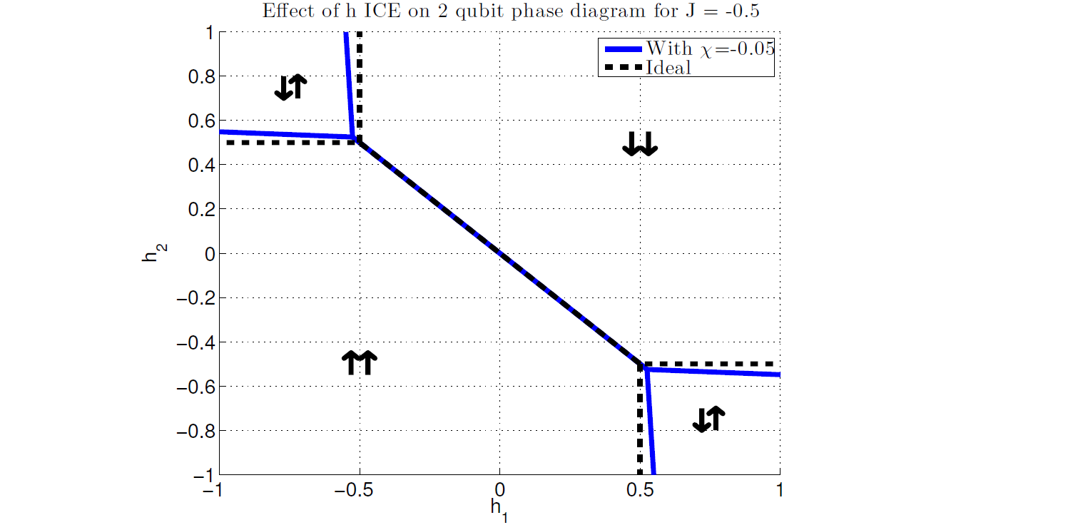
Fig. 126 Two-qubit (two Ising spin) phase diagram for \(J = -0.5\). The dashed lines show the locations of the expected phase boundaries between the four possible states of the system under the assumption of ideal Ising spin behavior. The solid lines show the locations of the phase boundaries for \(\chi = -0.05.\) To estimate the Ising spin parameters without systematic bias, \(\chi\) must be included in any model of the physical system. Data shown are representative of D-Wave 2X systems.

Given the form of the \(h\)-leakage terms, applying small adjustments to the \(h\) biases on the original problem can compensate somewhat for this error. However, \(\chi\) varies during the anneal (see Figure 123), and this correction corresponds to one specific point during the anneal. The single qubit freezeout point for typical anneal times occurs when \(s \approx 0.8\) and \(A(s)\) is around 100 MHz (see Figure 83). This is the last point in the anneal where any meaningful spin-flip dynamics occur; at that point \(\chi\) is approximately -0.015, so that value can, in principle, compensate for \(h\)-leakage. A better approach, however, is to choose \(\chi\) to correspond to a point earlier in the anneal—at or before the crossing point of \(A(s)\) and \(B(s)\). This is the localization point of a one-dimensional chain of spins.

Effective Two-Spin Systems For Larger Problems

Similar measurements may be repeated for larger problems made up of logical spins formed by strongly coupled groups of spins with strong intracluster coupling weights \(J_{cluster}\). Pairs of clusters are connected by the intercluster coupling weight \(J\), and the \(h_1\) and \(h_2\) weights are assigned to all spins in each cluster. These clusters freeze out at different anneal times depending on the number of spins and on coupling strengths \(J\) and \(J_{cluster}\), as shown in Figure 86 and Figure 87. These effective two-spin instances make it possible to probe ICE effects on \(h\) and \(J\) at different times during the anneal.

For each logical qubit size up to 6 (corresponding to 6+6 spins) held together with \(J_{\text{cluster}}=1\), ask the QPU to solve independent problems on the full-sized graph for varying \(J\), \(h_1\) and \(h_2\). Then fit the measured results to a fixed-temperature model of the phase diagram for the ideal problem—appropriately adjusted to the larger qubit counts, including the proper \(\chi\) contributions from the logical qubit components.

The dominant effects taken into account during the fitting to the phase diagram model are:

• The \(J\) realized may vary from the \(J\) requested. ICE effects on couplings characterized by \(\delta J\) are shown in Figure 121.

• With large-enough samples of logical two-spin problems, random \(\delta h\) errors cancel out; what remains is an offset field for each spin. This offset, \(h_{offset}\), characterizes the intrinsic flux offset of the logical qubit that is independent of \(h\).

• The difference between specified \(h\) and realized \(h\) may vary as described in the Distribution of h Scale Across Qubits section. Figure 127 shows the effect of this type of error on the phase diagram.

• Additional warping of the phase diagram occurs as \(\chi\) changes from \(-0.04\) to \(-0.015\) through anneal time \(s\).

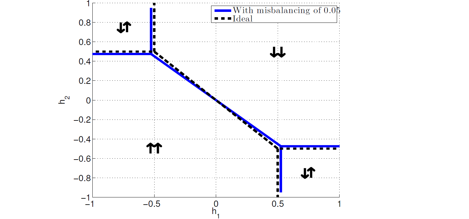
Fig. 127 Two-qubit (two Ising-spin) phase diagram for two spins of different magnitude (two qubits with different \(I_p\)) for a sample \(\chi\) value of \(J = -0.5\). The dashed lines show the locations of the expected phase boundaries between the four possible states of the system under the assumption of identical spin magnitudes. The solid lines show the locations of the phase boundaries for spin magnitudes that differ by \(0.05\). Data shown are representative of D-Wave 2X systems.

Characterizing the Effect of Flux Noise

This section characterizes the effects of flux noise on the quantum annealing process. The Error-Correction Features section describes the procedure that D-Wave uses to correct for drift.

Let there be a flux qubit biased at degeneracy \(h=0\) with tunneling energy \(\Delta_q\). Let the qubit be subject to flux noise with noise spectral density \(S_{\Phi}(f)\). If this qubit is subjected to experiments over a time interval \(t_{\rm exp}\), then it is subject to a random flux bias whose flux-flux correlator can be expressed as

\begin{equation} \left<\Phi_n(t)\Phi_n(0)\right> = \int_{f_{\rm min}}^{f_{\rm max}} df S_\Phi(f) \frac{\sin^2 2\pi f t}{(\pi f)^2} \end{equation}

where \(f_{\rm min} = 1/t_{\rm exp}\) and \(f_{\rm max} = \Delta_q/h\).[7]

[7]

The derivation of this expression follows the same logic as that for the phase-phase correlator given in Eq. 10c of Phys. Rev. B 67, 094510 (2003), albeit with an appropriate low-frequency cutoff.

The ambiguity with quantum annealing is in defining the appropriate choice of \(\Delta_q\), since this quantity is swept during an experiment. The value of \(\Delta_q\) should be the point in the anneal at which a given qubit localizes. For a single isolated qubit, the appropriate value of \(\Delta_q\) is on the order of the inverse decoherence time \(1/T_2^*\), where \(T_2^*\) is a function of \(\Delta_q\). Thus, \(\Delta_q\) becomes that of the coherent-incoherent crossover. For a system of coupled qubits, localization can occur at much larger values of \(\Delta_q\). In this case, the coupled qubit system can undergo a phase transition earlier in the anneal where the qubits are coherent. D-Wave QPUs realize these phase transitions at \(\Delta_q/h \sim 2\) GHz.

For example, the calculation of the fractional error in the dimensionless 1-local bias \(h_i\) proceeds as follows. Typical qubits experience low-frequency flux noise characterized by a noise spectral density of the form

\begin{equation} S_\Phi(f) = \frac{A}{f^\alpha} \end{equation}

with amplitude such that \({\sqrt S_\Phi ({\rm 1 Hz}) \sim 2 \mu\Phi_0/\sqrt{\rm Hz}}\) and exponent \(0.75 \leq \alpha < 1\). Given that the uncertainty in \(\alpha\) is large and a lack of experimental evidence that the form given above is valid up to frequencies of order \(\Delta_q/h \sim 2\) GHz, \(\alpha = 1\) is used in these calculations. Integrating this equation from \(f_{\rm min} = 1\) mHz to \(f_{\rm max} = 2\) GHz yields an integrated flux noise

\begin{equation} \delta \Phi_n = \sqrt{\int_{f_{\rm min}}^{f_{\rm max}} df S_\Phi(f)} \approx 10\ \mu\Phi_0. \end{equation}

A qubit with \(\Delta_q/h = 2\) GHz also possesses a persistent current \(|I_p| \approx 0.8\) \(\mu\)A. The maximum achievable antiferromagnetic coupling between a pair of qubits is \(M_{\rm AFM} \approx 2 \ {\rm pH}\). Thus, the scale of \(h\) is set by

\begin{equation} \Phi_h \equiv M_{\rm AFM} |I_p| \approx 0.8 \ {\rm m} \Phi_0. \end{equation}

The relative error in the dimensionless parameter \(h_i\) is then

\begin{equation} \delta h_i \equiv \frac{\delta \Phi_n}{\Phi_h} \approx 0.01. \end{equation}

Example of ICE Effects on Solution Quality

As discussed in the ICE section, the distributions \(\delta h\) and \(\delta J\) depend on annealing time \(t_f\) and vary with anneal fraction \(s\) during the anneal. Because \(\delta h\) and \(\delta J\) may vary with \(s\) (as well as with any errors in the ratio \(h/J\)), ICE can drive a system across a phase boundary—whether a quantum phase transition or a later classical phase transition.

Consider a simple two-spin problem with biases \(h_1 = h_2 = 0.01\) and \(J = -0.5\). You can expect to see spins \(\downarrow \downarrow\) (that is, \(s_1, s_2 = -1\)) in the problem solution. If \(\delta h\) is such that the QPU sees \(h_1, h_2 = -0.01\) early in the anneal, the system localizes in the \(\uparrow \uparrow\) state. Perhaps later, the effective ICE signal becomes smaller and the system crosses a phase boundary to prefer \(\downarrow \downarrow\). Depending on when this happens in relation to freezeout time, the system may or may not be able to respond:

• If \(\delta h\) changes early enough in the anneal, the system can respond and provide the correct answer.

• If \(\delta h\) occurs too late, the early ICE is effectively locked in and both spins remain up.

This example shows that there are two components to ICE: the final error on the classical Ising spin system defined by equation qpu_equation_ising_objective, and the rest of the error contributing to a variation in the anneal path on the way to the final classical Hamiltonian. Depending on problem details, either of these effects may dominate—exchanging roles earlier, later, or at multiple times in the anneal.

Other Error Sources

As well as the ICE effects discussed at length in the ICE section, a number of other factors may affect system performance, including temperature, high-energy photon flux, readout fidelity, programming errors, and spin-bath polarization. This section looks at each of these in turn. For guidance on how to work around some of these factors to get improved performance, see the QPU Configuration: Best Practices section.

Temperature

In a formal sense, temperature is defined for a system in thermodynamic equilibrium. In a practical sense, however, if the equilibrium time of a given subsystem is very short compared to the relaxation time between subsystems, then that subsystem may not be in thermal equilibrium with other subsystems capable of exchanging energy.

For example, the superconducting QPU and the block of metal attached to both it and a separate low-temperature thermometer have distinct temperatures. The thermometer measures the temperature of the dilution refrigerator’s mixing chamber; however, this may be a couple of millikelvin colder than the QPU. Furthermore, there is a distinction between the temperature of the quasiparticles in a superconducting wiring layer of the QPU and its phonons, and between the phonons of the wiring layer and those of the silicon substrate.

For timescales over which the annealing algorithm operates, the qubits are considered to be in equilibrium with a thermal bath at an effective temperature that can be measured, for example, by looking at the equilibrium distribution of single, uncoupled qubits when held in a fixed longitudinal and transverse field. (See Figure 83 and [Joh2011], Supplemental Information, section II.D page 8.)

Ensuring that a QPU operates at millikelvin-scale temperatures requires minimizing the amount of energy deposited on the QPU, as well as ensuring that energy is efficiently removed from it. Nevertheless, some heat is dissipated on the QPU during normal operation, particularly during the programming cycle. This can, depending on the frequency of programming, increase the effective temperature of the qubits and therefore affect solution quality.

Temperature effects vary from QPU to QPU, and depend on a number of manufacturing-related details. In practice, the effects can be quantified by performing the aforementioned equilibrium distribution tests when no programming is being performed and again when programming is done at maximum frequency, and then comparing the values.[8]

[8]

This corresponds to a case where many problems, each requesting only a small number of reads, are queued to run on the QPU.

Note

Contact D-Wave Customer Support to obtain the detailed properties of your system.

As a simple illustration of the effect of thermal equilibration, consider a single-qubit problem. As shown in Figure 86, you find that single qubits freeze out at an \(s\) value of roughly \(0.7\). At that point, \(B(s)\)—for the particular QPU shown—is approximately 7 GHz. Before this freezeout point, you can assume that the single qubits are in thermal equilibrium at some temperature \(T\) after which no further dynamics are present. At \(s = 0.7\), an applied \(h\) of \(1.0\) to the single qubit results in an energy difference between the up and down states of 7 GHz. The expected distribution for the spin up population is: \(P_{\uparrow} / 1-P_{\uparrow} = e^{-\delta E / k_b T}\).

Because \(\delta E = B(s) h\), you can sweep \(h\) over a small range and fit the result to a hyperbolic tangent and extract the resulting \(T\) of the QPU. Figure 128 shows the results of a measurement where you sweep the \(h\) values on all the qubits on a QPU, shift the curves to have the same centers, and then fit the averaged data to a hyperbolic tangent to extract the effective temperature of the qubits.

As a consequence, even when the temperature of the mixing chamber is constant, the effective temperature of the qubits may vary by a few millikelvin, depending on usage.

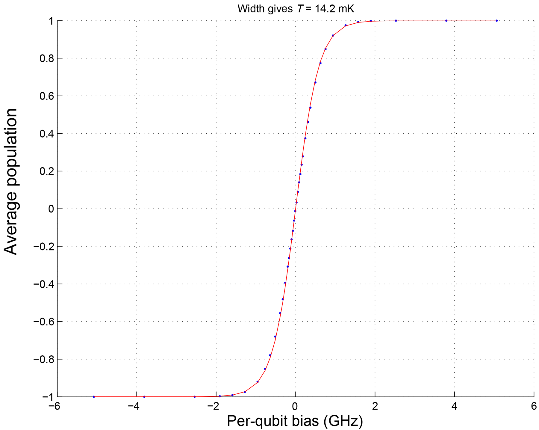
Fig. 128 Single qubit temperature extraction: Sampling the trivial 1-qubit problem, \(H = -h_i s_i\) on the QPU for qubit \(i\) (averaged over all qubits after centering each data set) for several values of \(h_i\) on the x-axis, results in the blue points shown in this plot. Fitting the data to a Boltzmann distribution gives the red curve and allows us to extract an effective temperature of \(14.2\) mK for this sample data. Conversion from \(h_i\) to energy bias is done by looking at the anneal schedule \(B(s)\) at the single qubit freezeout point in Figure 86.

High-Energy Photon Flux

The presence of relatively high-energy photons also plays a role. High-energy, in this context, means that photon energy and population exceed what would be expected at equilibrium at the measured effective qubit temperature.

These photons enter the QPU from higher-temperature stages through cryogenic filtering. When the annealing algorithm runs, they can cause transitions to much higher-energy problem states than would be expected given the equilibrium picture discussed in the previous section. Given a constant flux of high-energy photons, the probability of such a transition should increase the longer the annealing algorithm takes. This phenomenon may manifest as an appearance of solutions with energies much higher than the expected thermal distribution. This effect grows with longer anneal times.

Note

The anneal schedule feature discussed the Varying the Global Anneal Schedule section allows you to insert pauses at intermediate values of \(s\). Be aware that pausing at intermediate points in the quantum annealing process may increase the probability of transitions to higher energy states. As with the standard annealing schedule, the phenomenon may manifest as an appearance of solutions with energies much higher than the expected thermal distribution of energies and the effect grows with pause time.

Readout Fidelity

Readout fidelity is not typically a significant factor in the D-Wave quantum computer. Averaged over an ensemble of randomized bit strings, the typical readout fidelity of the system is greater than 99%. That is, one out of every 100 reads of a given problem may report a solution that is different from that found by the QPU by one or more bit flips.

For guidelines on how to use multiple reads to identify readout errors and make the best use of QPU time, see the QPU Configuration: Best Practices section.

Programming Errors

A problem that uses all available qubits and couplers has a greater than 90% chance of being programmed without error. Occasionally, however, programming (or reset) issues occur during the programming cycle of the QPU, moving the problem implementation on the QPU far enough away from the intended problem that the solutions computed by the QPU do not overlap the low-energy subspace of the intended problem. If low-energy answers for a single problem are critical, submit the problem at least twice.

Note

Spin-reversal transforms reprogram the system and thereby offer another way to reduce the impact of these errors; for more information on this technique, see the QPU Configuration: Best Practices section.

Spin-Bath Polarization Effect

One of the main sources of environmental noise affecting the qubit is magnetic fluctuations from an ensemble of spins local to the qubit wiring. This produces low-frequency flux noise that can cause the misspecification errors referred to in this document as “ICE 1.” In addition, the persistent current flowing in the qubit body during the quantum annealing algorithm produces a magnetic field that can partially align or polarize this ensemble of spins.

This partially polarized environment may bias the body of the qubit. This phenomenon may manifest, for example, in measurements of single qubit transition widths (the width of qubit population versus h bias). For very long anneal times, the polarized environment may add to the external h bias, producing a transition width that is narrower than the width expected from a thermal distribution. The partially polarized environment can also produce sample-to-sample correlations, biasing the QPU towards previously achieved spin configurations.

To reduce these sample-to-sample correlations, enable the reduce_intersample_correlation solver parameter. This setting adds optimal delay times before each anneal, giving the spin bath time to depolarize and thereby lose the effects from the previous read. It adds a delay that varies (approximately) between \(200\) microseconds and \(10\) milliseconds, increasing linearly with increasing length of the schedule:

\begin{equation} delay = 500 + \frac{\rm{T} (10000 - 500)}{2000} \end{equation}

where T is the total time of the anneal schedule.

Important

Enabling this parameter drastically increases problem run times. To avoid exceeding the maximum problem run time configured for your system, limit the number of reads when using this feature. For more information, see the Operation and Timing section.

The anneal schedule feature discussed in the Annealing Implementation and Controls chapter allows you to insert pauses at intermediate values of \(s\). Be aware that pausing at intermediate points in the quantum annealing process may increase the degree of polarization of the spin environment and thus the size of the bias back on the body of the qubit.

Error-Correction Features

D-Wave quantum computers provide some features to alleviate the effects of the errors described in previous chapters. Additionally, you can mitigate some effects through the techniques described in the Using the QPU sections.

Drift Correction

Flux noise is described and its effects characterized in the Flux Noise of the Qubits and Characterizing the Effect of Flux Noise subsections of the Errors and Error Correction section.

By default, the D-Wave system uses the following procedure to measure and correct for the longest drifts once an hour. You can disable the application of any correction by setting the flux_drift_compensation solver parameter to False. If you do so, you should apply flux-bias offsets manually; see the Calibration Refinement section.

1. The number of reads for a given measurement, \(N_\mathrm{reads}\), is set to 2000.

2. A measurement of the zero-problem, with all \(h_i = J_{i,j} = 0\) is performed, and the average spin computed for the \(i\)-th qubit according to \(\left<s_i\right> = \sum_j{s_i^{(j)}}/N_\mathrm{reads}\), where \(s_i^{(j)} \in \{+1,-1\}\) and the sum is performed over the \(N_\mathrm{reads}\) independent anneal-read cycles.

3. The flux offset drift of the \(i\)-th qubit is estimated as \(\delta\Phi_i = w_i\left<s_i\right>\), where \(w_i\) is the thermal transition width of qubit \(i\); defined below.

4. The measured \(\delta\Phi_i\) are corrected with an opposing on-QPU qubit flux–bias shift. The magnitude of the shift applied on any given iteration is capped to minimize problems due to (infrequent) large \(\delta\Phi_i\) measurement errors.

5. \(N_\mathrm{reads}\) is doubled, up to a maximum of 20,000.

6. The procedure repeats from step 2 at least 6 times. It repeats beyond 6 if the magnitude of any of the \(\delta\Phi_i\) after the last iteration is significantly larger than the expected variation due to \(1/f\) flux noise.

The thermal width, \(w_i\), of qubit \(i\) is determined during QPU calibration by measuring the isolated qubit (\(J_{i,j} = 0\) everywhere) average spin \(\left<s_i(\Phi_i^{(x)})\right>\) as a function of applied flux bias \(\Phi_i^{(x)}\) for each qubit, and fitting to the expression \(\tanh{\left[(\Phi_i^{(x)}-\Phi_i^{(0)})/w_i\right]}\), where \(\Phi_i^{(0)}\) and \(w_i\) are fit parameters.

For a typical \(w_i\) of order 100 \(\mu\Phi_0\), statistical error is measured at \(100~\mu\Phi_0/\sqrt{20000} \simeq 1~\mu\Phi_0\). This is much smaller than the root mean square (RMS) flux noise, which is on the order of 10 \(\mu\Phi_0\) for the relevant time scales.

Extended \(J\) Range

Ising minimization problems that the D-Wave system solves may require that the model representing a problem be minor-embedded on the working graph, a process that involves creating qubit chains to represent logical variables, as introduced in the Minor Embedding section. In an embedding, intra-chain qubit couplings must be strong compared to the input couplings between the chains.

Most discussions of chain strength involve the ratio of two absolute values:

• Chain coupling strength—Magnitude of couplings between qubits in a chain

• Problem scale—Maximum magnitude of couplings among qubits (physical or logical) in a problem

that is,

\begin{equation} \frac{chain\_coupling\_strength}{problem\_scale}. \end{equation}

For example, if all of the chains have \(J\) values of \(-1\), and the rescaled[9] logical problem has \(J\) values of \(- \frac{1}{4}\) to \(+ \frac{1}{4}\), you say that the chain strength is \(4\). Likewise, if the chains have \(J\) values of \(-2\), and the rescaled logical problem has \(J\) values of \(- \frac{1}{2}\) to \(+ \frac{1}{2}\), again you say that the chain strength is \(4\).

[9]

See the description of the auto_scale solver parameter in the QPU Solver Parameters section.

Because the range of coupling strengths available is finite, chaining is typically accomplished by setting the coupling strength to the largest allowed negative value and scaling down the input couplings relative to that. Yet a reduced energy scale for the input couplings may make it harder for the QPU to find global optima for a problem.

To address this issue, some solvers support stronger chain couplings through an extended_j_range solver property. Because embedded problems typically have chain couplings that are at least twice as strong as the other couplings, and standard chain couplings are all negative, this feature effectively doubles the energy scale available for embedded problems; see Figure 129.

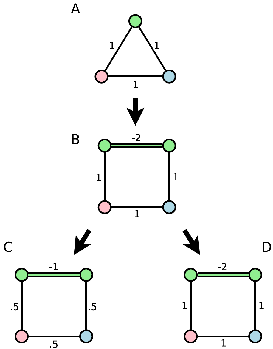
Fig. 129 Embedding an input that does not fit directly on a D-Wave QPU. The original problem (A) has a green vertex that is replaced by a chain of two vertices connected with a ferromagnetic coupling (B). With the standard coupling range, the embedded problem must be scaled down for the QPU, which can lead to decreased performance (C). However, with an extended coupling range, no rescaling is necessary (D).

Using the available larger negative values of \(J\) increases the dynamic \(J\) range. On embedded problems, which use strong chains of qubits to build the underlying graph, this increased range means that the problem couplings are less affected by ICE and other effects. However, strong negative couplings can bias a chain and therefore flux-bias offsets might be needed to recalibrate it to compensate for this effect; see the Calibration Refinement section for more information.

Calibration Refinement

In an optimal QPU calibration, annealing unbiased qubits produces spin-state statistics that are equally split between spin-up and spin-down. When plotted against the \(h\) values, this even distribution results in a sigmoid curve that passes through the point of origin (0,0). However, non-idealities in QPU calibration and coupling to its environment result in some asymmetry. This asymmetry typically increases under strong coupling (such as when the extended_j_range is used for chains): a \(J\)-induced bias (an offset magnetic field that is potentially \(s\)-dependent).[10]. hese effects shift the sigmoid curve of plotted \(h\) values from its ideal path, as shown in Figure 130.

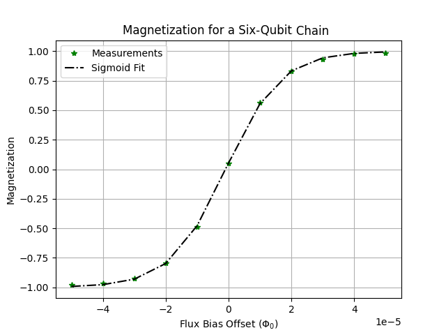
Fig. 130 Magnetization (mean spin value) of a six-qubit chain on an Advantage2™ QPU as a function of applied per-qubit flux-bias offset. A sigmoid function (\(\tanh()\), the dashed line) fit to the measurements intersects the horizontal grid line slightly above the zero.

[10]

This offset occurs because of the higher susceptibility of the tunable coupler [Har2009].

While the effect may be minor for many optimization problems, for others, such as material simulation, it may be significant. You can compensate by refining the calibration, applying per-qubit flux_biases to nudge the plotted \(h\) sigmoid to its ideal position.

Flux biases can be used to refine the standard calibration. [Che2023] describes (and links to code) techniques that tune the Hamiltonian to reduce the differences between the symmetric ideal and the asymmetric measurements on the QPU.

Note

The applied flux bias is constant in time (and \(s\)), but it appears in the Hamiltonian shown in equation (2) as a term \(I_p \phi_{\rm flux bias} \sigma_z\)—the applied energy grows as \(\sqrt{B(s)}\). An applied flux bias is different from an applied \(h\); do not use one to correct an error in the other.

Virtual Graphs

Important

The virtual graph feature is deprecated due to improved calibration of newer QPUs: Ocean software’s VirtualGraphComposite class will be removed in a future release. To calibrate chains for residual biases, follow the instructions in [Che2023].

The D-Wave virtual graph feature (see the VirtualGraphComposite class) simplifies the process of minor-embedding by enabling you to more easily create, optimize, use, and reuse an embedding for a given working graph. When you submit an embedding and specify a chain strength using these tools, they automatically calibrate the qubits in a chain to compensate for the effects of biases that may be introduced as a result of strong couplings. For more information on virtual graphs, see Virtual Graphs for High-Performance Embedded Topologies, D-Wave White Paper Series, no. 14-1020A, 2017. This and other white papers are available from https://www.dwavesys.com/resources/publications.

Virtual graphs make use of Extended J Range and Calibration Refinement features. These controls allow chains to behave more like physical qubits on the working graph, thereby improving the performance of embedded sampling and optimization problems.

Note

Despite the similarity in name, the virtual graphs feature is unrelated to D-Wave’s virtual full-yield chip (VFYC) solver.

Whether virtual graph features are available may vary by solver; check for the extended_j_range property to see if it is present and what the range is. (The j_range property is unchanged.) When using an extended \(J\) range, be aware that there are additional limits on the total coupling per qubit: the sum of the \(J\) values for each qubit must be in the range specified by the per_qubit_coupling_range solver property.

Flux-biases are set through the flux_biases parameter, which takes a list of doubles (floating-point numbers) of length equal to the number of working qubits. Flux-bias units are \(\Phi_0\); typical values needed are \(< 10^{-4} \ \Phi_0\). Maximum allowed values are typically \(> 10^{-2} \ \Phi_0\). The minimum step size is smaller than the typical levels of intrinsic \(1/f\) noise; see the Characterizing the Effect of Flux Noise section.

Note

By default, the D-Wave system automatically compensates for flux drift as described in the Characterizing the Effect of Flux Noise section. If you choose to disable this behavior, you should apply flux-bias offsets manually through the flux_biases parameter.

Be aware of the following points when using virtual graph features:

• Autoscaling is not supported with flux-bias offsets. When you use this feature, autoscaling is automatically disabled by default, unlike in the usual system behavior.

• The \(J\) value of every coupler must fall within the range advertised by the extended_j_range property.

• The sum of all the \(J\) values of the couplers connected to a qubit must fall within the per_qubit_coupling_range property. For example, if this property is [-9.0 6.0], the following \(J\) values for a six-coupler qubit are permissible:

  \[1, 1, 1, 1, 1, 1,\]

  where the sum is \(6\), and also

  \[1, 1, 1, -2, -2, -2,\]

  where the sum is \(-3\). However, the following values, when summed, exceed the range and therefore are impermissible:

  \[-2, -2, -2, -2, -2, -2.\]

• While the extended \(J\) range in principle allows you to create almost arbitrarily long chains without breakage, the maximum chain length where embedded problems work well is expected to be in the range of 5 to 7 qubits.

• When embedding logical qubits using the extended \(J\) range, limit the degree, \(D\), of each node in the logical qubit tree to

  \begin{equation} \begin{array}{rcl} D &=& {\rm floor} \bigg[ \frac{\min(per\_qubit\_coupling\_range)}{\min(extended\_j\_range) - \min(j\_range)} \\ & & -\frac{num\_couplers\_per\_qubit \times \min(j\_range)} {\min(extended\_j\_range) - \min(j\_range)} \bigg] \end{array} \end{equation}

  where \(num\_couplers\_per\_qubit = 5\) for the Advantage™ QPU; see the QPU Architecture section.