

Stating the Problem#
Once properly stated, a problem can be formulated as an objective function to be solved on a D‑Wave solver.
D‑Wave provides several resources containing many reference examples:
Ocean software’s collection of code examples on GitHub.
D-Wave papers (for example, [dwave2]) and links to user applications.
This section provides a sample of problems in various fields, and the available resources for each (at the time of writing); having a relevant reference problem may enable you to use similar solution steps when solving your own problems on D‑Wave solvers.
Many of these are discrete optimization, also known as combinatorial optimization, which is the optimization of an objective function defined over a set of discrete values such as Booleans.
Keep in mind that there are different ways to model a given problem; for example, a constraint satisfaction problem (CSP) can have various domains, variables, and constraints. Model selection can affect solution performance, so it may be useful to consider various approaches.
Problem |
Beginner Content Available? |
Solvers |
Content |
|---|---|---|---|
QPU, hybrid |
Code, papers |
||
QPU |
Papers |
||
QPU |
Papers |
||
Yes |
QPU |
Code, papers |
|
QPU, hybrid |
Papers |
||
Yes |
QPU, hybrid |
Code, papers |
|
QPU |
Papers |
||
Yes |
QPU, hybrid |
Code, paper |
|
QPU |
Papers |
||
Yes |
QPU, hybrid |
Code, papers |
|
QPU, hybrid |
Papers |
Whether or not you see a relevant problem here, it’s recommended you check out the examples in D‑Wave’s collection of code examples and corporate website for the latest examples of problems from all fields of study and industry.
Circuits & Fault Diagnosis#
Fault diagnosis attempts to quickly localize failures as soon as they are detected in systems such as sensor networks, process monitoring, and safety monitoring. Circuit fault diagnosis attempts to identify failed gates during manufacturing, under the assumption that gate failure is rare enough that the minimum number of gates failing is the most likely cause of the detected problem.
The Example Reformulation: Circuit Fault Diagnosis section in the Reformulating a Problem chapter shows the steps of solving a circuit fault diagnosis problem on a D‑Wave QPU.
Code Examples#
Logic Circuit: Embedding Effects
Solves a logic circuit problem using Ocean tools to demonstrate solving a CSP on a D‑Wave QPU solver.
-
Demonstrates the use of D‑Wave solvers to solve a three-bit multiplier circuit.
-
Verifies equivalence of two representations of electronic circuits using a discrete quadratic model (DQM).
Papers#
[Bia2016] discusses embedding fault diagnosis CSPs on the D‑Wave system.
[Bis2017] discusses a problem of diagnosing faults in an electrical power-distribution system.
[Pap1976] discusses decomposing complex systems for the problem of generating tests for digital-faults detection.
[Per2015] maps fault diagnosis to a QUBO and embeds onto a QPU.
Computer Vision#
Computer vision develops techniques to enable computers to analyse digital images, including video. The field has applications in industrial manufacturing, healthcare, navigation, miltary, and many other areas.
Papers#
[Arr2022] compares quantum and classical approaches to motion segmentation.
[Bir2021] discusses a quantum algorithm for solving a synchronization problem, specifically permutation synchronization, a non-convex optimization problem in discrete variables.
[Gol2019] derive an algorithm for correspondence problems on point sets.
[Li2020] translates detection scores from bounding boxes and overlap ratio between pairs of bounding boxes into QUBOs for removing redundant object detections.
[Ngu2019] demonstrates good prediction performance of a regression algorithm for a lattice quantum chromodynamics simulation data using a D‑Wave 2000Q system.
Database Queries (SAT Filters)#
A satisfiability (SAT) filter is a small data structure that enables fast querying over a huge dataset by allowing for false positives (but not false negatives).
Papers#
Factoring#
The factoring problem is to decompose a number into its factors. There is no known method to quickly factor large integers—the complexity of this problem has made it the basis of public-key cryptography algorithms.
Code Examples#
-
Demonstrates the use of D‑Wave QPU solvers to solve a small factoring problem.
-
Demonstrates the use of D‑Wave QPU solvers to solve a small factoring problem.
Papers#
[Dri2017] investigates prime factorization using quantum annealing and computational algebraic geometry, specifically Grobner bases.
[Dwave3] discusses integer factoring in the context of using the D‑Wave Anneal Offsets feature; see also the Anneal Offsets section.
[Bur2002] discusses factoring as optimization.
[Jia2018] develops a framework to convert an arbitrary integer factorization problem to an executable Ising model.
[Lin2021] applies deep reinforcement learning to configure adiabatic quantum computing on prime factoring problems.
Finance#
Portfolio optimization is the problem of optimizing the allocation of a budget to a set of financial assets.
Papers#
[Coh2020] investigates the use of quantum computers for building an optimal portfolio.
[Coh2020b] analyzes 3,171 US common stocks to create an efficient portfolio.
[Das2019] provides a quantum annealing algorithm in QUBO form for a dynamic asset allocation problem using expected shortfall constraint.
[Din2019] seeks the optimal configuration of a supply chain’s infrastructures and facilities based on customer demand.
[Els2017] discusses using Markowitz’s optimization of the financial portfolio selection problem on the D‑Wave system.
[Gra2021] uses portfolio optimization as a case study by which to benchmark quantum annealing controls.
[Kal2019] explores how commercially available quantum hardware and algorithms can solve real world problems in finance.
[Mug2020] implements dynamic portfolio optimization on quantum and quantum-inspired algorithms and compare with D‑Wave hybrid solvers.
[Mug2021] proposes a hybrid quantum-classical algorithm for dynamic portfolio optimization with minimal holding period.
[Oru2019] looks at forecasting financial crashes.
[Pal2021] implement in a simple way some complex real-life constraints on the portfolio optimization problem
[Phi2021] selects a set of assets for investment such that the total risk is minimised, a minimum return is realised and a budget constraint is met.
[Ros2016a] discusses solving a portfolio optimization problem on the D‑Wave system.
[Ven2019] investigates a hybrid quantum-classical solution method to the mean-variance portfolio optimization problems.
Graph Partitioning#
Graph partition is the problem of reducing a graph into mutually exclusive sets of nodes.
Code Examples#
-
Solves a graph partitioning problem on a QPU.
-
Solves a graph partitioning problem using the DQM solver in the Leap service.
-
Solves a maximum cut problem on a QPU.
-
Identifies clusters in a data set.
-
Fragments a population into separate groups via a “separator” using the DQM solver in the Leap service.
Papers#
[Bod1994] investigates the complexity of the maximum cut problem.
[Gue2018] performs simulations of the Quantum Approximate Optimization Algorithm (QAOA) for maximum cut problems.
[Hig2022] computes core-periphery partition for an undirected network formulated as a QUBO problem.
[Jas2019] proposes a using quantum annealing on extreme clustering problems.
[Ush2017] discusses unconstrained graph partitioning as community clustering.
[Zah2019] proposes an algorithm to detect multiple communities in a signed graph.
Machine Learning#
Artificial intelligence (AI) is transforming the world. You see it every day at home, at work, when shopping, when socializing, and even when driving a car. Machine learning algorithms operate by constructing a model with parameters that can be learned from a large amount of example input so that the trained model can make predictions about unseen data.
Most of the transformation that AI has brought to-date has been based on deterministic machine learning models such as feed-forward neural networks. The real world, however, is nondeterministic and filled with uncertainty. Probabilistic models explicitly handle this uncertainty by accounting for gaps in our knowledge and errors in data sources.
A probability distribution is a mathematical function that assigns a probability value to an event. Depending on the nature of the underlying event, this function can be defined for a continuous event (e.g., a normal distribution) or a discrete event (e.g., a Bernoulli distribution). In probabilistic models, probability distributions represent the unobserved quantities in a model (including noise effects) and how they relate to the data. The distribution of the data is approximated based on a finite set of samples. The model infers from the observed data, and learning occurs as it transforms the prior distributions, defined before observing the data, into posterior distributions, defined afterward. If the training process is successful, the learned distribution resembles the actual distribution of the data to the extent that the model can make correct predictions about unseen situations—correctly interpreting a previously unseen handwritten digit, for example.
In short, probabilistic modeling is a practical approach for designing machines that:
Learn from noisy and unlabeled data
Define confidence levels in predictions
Allow decision making in the absence of complete information
Infer missing data and latent correlations in data
Machine learning algorithms operate by constructing a model with parameters that can be learned from a large amount of example input so that the trained model can make predictions about unseen data.
Boltzmann Distribution#
A Boltzmann distribution is an energy-based discrete distribution that defines probability, \(p\), for each of the states in a binary vector.
Assume \(\vc{x}\) represents a set of \(N\) binary random variables. Conceptually, the space of \(\vc{x}\) corresponds to binary representations of all numbers from 0 to \(2^N - 1\). You can represent it as a column vector, \(\vc{x}^T = [x_1, x_2, \dots, x_N]\), where \(x_n \in \{0, 1\}\) is the state of the \(n^{th}\) binary random variable in \(\vc{x}\).
The Boltzmann distribution defines a probability for each possible state that \(\vc{x}\) can take using[1]
where \(E(\vc{x};\theta)\) is an energy function parameterized by \(\theta\), which contains the biases, and
is the normalizing coefficient, also known as the partition function, that ensures that \(p(\vc{x})\) sums to 1 over all the possible states of \(x\); that is,
Note that because of the negative sign for energy, \(E\), the states with high probability correspond to states with low energy.
The energy function \(E(\vc{x};\theta)\) can be represented as a QUBO: the linear coefficients bias the probability of individual binary variables in \(\vc{x}\) and the quadratic coefficients represent the correlation weights between the elements of \(\vc{x}\). The D‑Wave architecture, which natively processes information through the Ising/QUBO models (linear coefficients are represented by qubit biases and quadratic coefficients by coupler strengths), can help discrete energy-based machine learning.
Sampling from the D‑Wave QPU#
Sampling from energy-based distributions is a computationally intensive task that is an excellent match for the way that the D‑Wave system solves problems; that is, by seeking low-energy states. Samples from the D‑Wave QPU can be obtained quickly and provide an advantage over sampling from classical distributions.
When training a probabilistic model, you need a well-characterized distribution; otherwise, it is difficult to calculate gradients and you have no guarantee of convergence. While both classical Boltzmann and quantum Boltzmann distributions are well characterized, all but the smallest problems solved by the QPU should undergo postprocessing to bring them closer to a Boltzmann distribution; for example, by running a low-treewidth postprocessing algorithm.
Temperature Effects#
As in statistical mechanics, \(\beta\) represents inverse temperature: \(1/(k_B T)\), where \(T\) is the thermodynamic temperature in kelvin and \(k_B\) is Boltzmann’s constant.
The D‑Wave QPU generally operates at cryogenic temperatures below \(20\) mK, which can be translated to a scale parameter \(\beta\). The effective value of \(\beta\) varies from QPU to QPU and in fact from problem to problem since the D‑Wave QPU samples are not Boltzmann and time-varying phenomena may affect samples. Therefore, to attain Boltzmann samples, run the Gibbs chain for a number of iterations starting from quantum computer samples. The objective is to further anneal the samples to the correct temperature of interest \(T = 1/{\beta}\), where \(\beta = 1.0\).
In the D‑Wave software, postprocessing refines the returned solutions to target a Boltzmann distribution characterized by \(\beta\), which is represented by a floating point number without units. When choosing a value for \(\beta\), be aware that lower values result in samples less constrained to the lowest energy states. For more information on \(\beta\) and how it is used in the sampling postprocessing algorithm, see the Postprocessing section.
Probabilistic Sampling: RBM
A restricted Boltzmann machine (RBM) is a special type of Boltzmann machine with a symmetrical bipartite structure; see Figure 153.
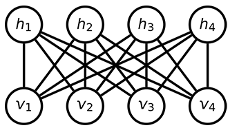
Fig. 153 Bipartite structure of an RBM, with a layer of visible variables connected to a layer of hidden variables.#
It defines a probability distribution over a set of binary variables that are divided into visible (input), \(\vc{v}\), and hidden, \(\vc{h}\), variables, which are analogous to the retina and brain, respectively.[2] The hidden variables allow for more complex dependencies among visible variables and are often used to learn a stochastic generative model over a set of inputs. All visible variables connect to all hidden variables, but no variables in the same layer are linked. This limited connectivity makes inference and therefore learning easier because the RBM takes only a single step to reach thermal equilibrium if you clamp the visible variables to particular binary states.
During the learning process, each visible variable is responsible for a feature from an item in the dataset to be learned. For example, images from the famous MNIST dataset of handwritten digits[3] have 784 pixels, so the RBMs that are training from this dataset require 784 visible variables. Each variable has a bias and each connection between variables has a weight. These values determine the energy of the output.
Without the introduction of hidden variables, the energy function \(E(\vc{x})\) by itself is not sufficiently flexible to give good models. You can write \(\vc{x}=[\vc{v},\vc{h}]\) and denote the energy function as \(E(\vc{v},\vc{h})\).
Then,
\begin{equation} p(\vc{x};\theta) = p(\vc{v},\vc{h};\theta) \end{equation}and of interest is
\begin{equation} p(\vc{v};\theta) = \sum_\vc{h} p(\vc{v},\vc{h};\theta), \end{equation}which you can obtain by marginalizing over the hidden variables, \(\vc{h}\).
A standard training criterion used to determine the energy function is to maximize the log likelihood (LL) of the training data—or, equivalently, to minimize the negative log likelihood (NLL) of the data. Training data is repetitively fed to the model and corresponding improvements made to the model.
When training a model, you are given \(D\) training (visible) examples \(\vc{v}^{(1)}, ..., \vc{v}^{(D)}\), and would like to find a setting for \(\theta\) under which this data is highly likely. Note that \(n^{th}\) component of the \(d^{th}\) training example is \(v_n^{(d)}\).
To find \(\theta\), maximize the likelihood of the training data:
The likelihood is \(L(\theta) = \prod_{d=1}^D p(v^{(d)};\theta)\)
It is more convenient, computationally, to maximize the log likelihood:
\begin{equation} LL(\theta)=log(L(\theta))=\sum_{d=1}^D {\log}p(v^{(d)};\theta). \end{equation}You can use the gradient descent method to minimize the \(NLL(\theta)\):
Starting at an initial guess for \(\theta\) (say, all zero values), calculate the gradient (the direction of fastest improvement) and then take a step in that direction.
Iterate by taking the gradient at the new point and moving downhill again.
To calculate the gradient at a particular \(\theta\), evaluate some expected values: \(E_{p(\vc{x};\theta)} f(\vc{x})\) for a set of functions \(f(\vc{x})\) known as the sufficient statistics. The expected values cannot be determined exactly, because you cannot sum over all \(2^N\) configurations; therefore, approximate by only summing over the most probable configurations, which you can obtain by sampling from the distribution given by the current \(\theta\).
Energy-Based Models
Machine learning with energy-based models (EBMs) minimizes an objective function by lowering scalar energy for configurations of variables that best represent dependencies for probabilistic and nonprobabilistic models.
For an RBM as a generative model, for example, where the gradient needed to maximize log-likelihood of data is intractable (due to the partition function for the energy objective function), instead of using the standard Gibbs’s sampling, use samples from the D‑Wave system. The training will have steps like these: a. Initialize variables. b. Teach visible nodes with training samples. c. Sample from the D‑Wave system. d. Update and repeat as needed.
Support Vector Machines
Support vector machines (SVM) find a hyperplane separating data into classes with maximized margin to each class; structured support vector machines (SSVM) assume structure in the output labels; for example, a beach in a picture increases the chance the picture is of a sunset.
Boosting
In machine learning, boosting methods are used to combine a set of simple, “weak” predictors in such a way as to produce a more powerful, “strong” predictor.
Generative and Discriminative Modeling#
Generative modeling is concerned with modeling the joint distribution of random variables \(X, Y\), whereas discriminative modeling is concerned with the conditional distribution of \(X \mid Y\).
Generative modeling with annealing quantum computers can be modeled by Boltzmann machines and quantum Boltzmann machines [Ami2018], [Ack1985]—families of learnable probability models over binary data.[4]
Discriminative modeling with annealing quantum computers can be modeled using both Boltzmann machines and quantum neural networks [Kak1995], [Chr1995].
Boltzmann Machines: Quantum Generalization#
Boltzmann machines model high-dimensional binary data. A Boltzmann machine is defined by its probability mass function,
where \(x \in \{\pm 1\}^n\) for some dimension \(n\), \(\theta \in \mathbb{R}^{n+n(n-1)/2}\) are the model parameters, and \(T: \{\pm 1\}^n \mapsto \{\pm 1\}^{n+n(n-1)/2}\) is the sufficient statistic [Wai2008] of the model; i.e.,
More generally, given a graph \(G=(V, E)\), you can define a graph-restricted Boltzmann machine specified by \(G\) to have sufficient statistics defined by,
where \(v_i \in V\) for \(i \in \{1, \dots, \lvert V\rvert\}\), and \(z_{e_i} = x_{e_{i_1}}x_{e_{i_2}}\), \(e_i = (e_{i_1}, e_{i_2}) \in E\) for \(i \in \{1, \dots, \lvert E \rvert \}\), and \(\theta \in \mathbb{R}^{\lvert V \rvert + \lvert E \rvert}\).
When only a subset of variables are observed, denoted \(v\), the remaining unobserved variables are referred to as hidden units \(h\). The marginal distribution of observed variables can be far more expressive due to the marginalization of hidden units; i.e.,
The inclusion of hidden units can potentially introduce challenges to be discussed in the Opportunities and Limitations section.
Given a binary dataset, one can fit a Boltzmann machine to the model using, for example, maximum likelihood estimates [Cas2002]. However, the maximum likelihood estimate for a Boltzmann machine is nontrivial to evaluate. The standard approach [Hin2002], [Ack1985] is to optimize the model using stochastic gradient descent [Boy2004].
The gradient of the log likelihood function itself is intractable:
Its intractability stems from the expectation term, with respect to the model, which requires an evaluation of the partition function \(Z(\theta)\). This motivates the need for Monte Carlo algorithms [Rob2004]; i.e., sample approximations of the expectation.
Sampling from Boltzmann machines is notoriously difficult and is where the annealing quantum computer excels.
The restricted Boltzmann machine [Hin2002], [Smo1986] is a special case of the graph-restricted Boltzmann machine in which the graph is a complete bipartite graph. Furthermore, partial observations are restricted to be on one and only one partite set of the graph. These modeling constraints were motivated by the need for an efficient training algorithm [Hin2002], [Hin2010].
Quantum Boltzmann machines offer a generalization of Boltzmann machines and are defined by Hamiltonians.
In D-Wave’s implementation, these Hamiltonians take the form:[5]
where the product \(\bigotimes\) denotes the Kronecker product [Str2012]. The probability measure is now defined by the diagonal elements of the density matrix,
To gain an intuitive understanding, consider a diagonal Hamiltonian—diagonal Hamiltonian (\(\gamma_i = 0\) for all \(i\)) corresponds to the classical definition of a Boltzmann machine. By construction of the Hamiltonian, the summation over \(Z_i\) and \(Z_iZ_j\) matrices result in a matrix whose diagonal entries correspond to each of the \(2^{\lvert V\rvert}\) binary strings’ probability (when normalized). When qubits are measured in the \(z\)-basis, or with respect to each \(Z_i\), binary strings are observed with their corresponding probabilities. The quantum Boltzmann machine can be trained using the same expressions or quantities used in classical Boltzmann machines, albeit based on a lower bound of the log likelihood [Ami2018].
Quantum Boltzmann Machines: Applications#
Applying arbitrary graph-restricted Boltzmann machines to real-world applications raises at least two challenges.
Data are seldom natively binary. For example, image data are continuous and text data are categorical.
Correlations are not guaranteed to be local and quadratic even when data are binary, thereby limiting the expressivity and goodness-of-fit of graph-restricted Boltzmann machines.
Identifying a mapping of input variables to model variables is at least as difficult as the quadratic assignment problem [Law1963]—an NP-hard problem. The problem can be formulated as maximizing the likelihood function over both mappings and parameters.
Both challenges can be addressed via several approaches. One solution is to leverage variants of (variational) autoencoders [Sch2015], [Bal1987], [Kin2013], for example, [Rol2016], [Li2016], [Zha2017], [Van2017], [Jan2016], [Kho2018]. The idea underpinning these approaches is to enforce a discrete-latent-space constraint in the model.
Defining variational autoencoders [Kin2013] with discrete latent variables is not a problem because the reparameterization trick [Kin2013] is not limited to real-valued random variables [Rol2016]. However, a problem arises in training such a discrete model via gradient descent: gradients are zero for discrete random variables. [Rol2016] addresses this training problem by augmenting binary latent variables with real-valued random variables. The auxiliary variables are equipped with distributions conditioned on the binary variables, resulting in nonzero gradients in backpropagation [Sch2015].
For example, consider the random variable \(Z \mid B\) where \(B\) is a Bernoulli random variable and \(Z \mid B = 0\) is \(0\), and \(Z \mid B = 1 \sim \text{Exponential}(1)\).
Using the inverse conditional distribution function (CDF) sampling method [Rob2004], you have,
where \(u\) is the noise variable, \(x\) is the encoded data input, and the second case for \(f\) comes from the inverse CDF of the exponential distribution. Because \(f\) is differentiable with nonzero gradients, one can meaningfully backpropagate through the discretization layer.
Another approach to modeling data with binary random variables is to use approximations proposed by [Jan2016], [Mad2016]. The approach is based on a limiting argument with annealed Gumbel distributions combined with a straight-through estimator [Ben2013],
where \(K\) represents the number of discrete values (\(K=2\) for binary) and \(\tau\) is an annealing parameter. When \(\tau \to 0\), \(z\) becomes a one-hot vector; i.e., \(z_i = 1\) for some index \(i\) and \(0\) for all other indices not equal to \(i\).
In a recent molecular-design application, [Kun2026] leveraged ideas from the neural hash function of [Eri2015] to discretize data. The binarization strategy applied in [Eri2015] penalizes the encoding network, during training, when latent variables deviate from \(\pm 1\). That is, the following loss function is added as a regularizer to the neural network training objective:
Finally, REINFORCE [Wil1992], [Gly1990] can also be used to backpropagate gradients through discretization layers,
A drawback of REINFORCE is that the estimator is effectively computed by expressions akin to finite differences, resulting in high variance. Bespoke variance-reduction techniques [Rob2004] are often required to stabilize the estimator. See [Jan2016] for a summary of relevant variance-reduction techniques based on control variates.
Boltzmann machines can also be used as discriminative models or, equivalently, used for modeling conditional distributions \(Y \mid X\). See [Cal2019] for an applied example using annealing quantum computers. Training of Boltzmann machines for discriminative tasks is no different from training generative models. Variables \(X\) and \(Y\) are both assigned to variables of a Boltzmann machine during training.[6]
At inference, however, only variables associated with \(X\) are fixed at their observed value and predictions are computed by sampling \(Y\mid X\). In practice, discriminative modeling with sparse graph-restricted Boltzmann machines poses a subtle variable-assignment problem, which is discussed in the Opportunities and Limitations section.
Quantum Neural Networks#
Quantum neural networks ([Kak1995], [Chr1995]) are families of functions evaluated via parameterized quantum systems.[7] That is, a quantum neural network, \(f_\theta\), parameterized by \(\theta\) is defined as
where \(x \in \mathbb{R}^d\) represents input data, \(U_\theta\) represents a unitary transformation, \(U_\theta^\dagger\) its conjugate transpose, \(\lvert \psi_0 \rangle\) is an initial state of the system, \(\langle \psi_0 \rvert\) its conjugate transpose, and \(\hat F\) is a quantum observable.
Essentially, a quantum neural network is a parameterized function whose outputs are expected values of the quantum system. A difficulty in applying quantum neural networks to real-world applications is in training. Evaluating or even approximating gradients of a loss function with respect to the network parameters is nontrivial due to the intractability of densities and expectations. Much of the literature on training quantum neural networks has been dedicated to gate-model systems, using, for example, the parameter-shift rule and its generalizations [Mit2018], [Wie2022].
A more relevant approach to training quantum annealing-based neural networks is via equilibrium propagation [Sce2017], a gradient-estimation technique originally introduced in the context of training energy-based models [Teh2003]. Generalizations to quantum equilibrium propagation have been proposed in [Mas2025], [Sce2024]. The parameter update rule can be described as follows.
Consider an example Hamiltonian of the form,
where \(Z_i\) are as defined in the Boltzmann Machines: Quantum Generalization section, \(J_{i,j}, h_i\) are scalar functions of the input data \(x\); that is, \(h_i: \mathbb{R}^d \mapsto \mathbb{R}\) and \(J_{i, j}:\mathbb{R}^d \mapsto \mathbb{R}\). Note \(h_i\) and \(J_{i, j}\) include constant functions independent of \(x\). Equilibrium propagation approximates the gradients by introducing another Hamiltonian, a nudge Hamiltonian, defined as
where \(y \in \mathbb{R}^{d_2}\) are the desired network outputs, and \(\tilde h_i\) is similarly defined to \(h\), \(\tilde h_i: \mathbb{R}^d \mapsto \mathbb{R}\). The gradient is expressed as
where \(S, S'\) are spin-valued random vectors with distribution prescribed by \(H(x), H_\text{nudge}(x, y)\) respectively, \(\theta = (h, J)\) (as defined in the Boltzmann Machines: Quantum Generalization section), \(T\) is the sufficient statistic of \(H\) (as defined in the same section), and \(C: \mathbb{R}^{|V| + |E|} \times \mathbb{R}^d \times \mathbb{R}^{d_2} \mapsto \mathbb{R}\) is a differentiable cost function (with respect to the first argument). The gradient, expressed as a difference of expectations, can be readily estimated by sampling from a quantum computer.
The applicability of quantum annealing-based neural networks has been demonstrated in MNIST [Den2012] image classification tasks [Zha2025], [Lay2024]. Notably, [Lay2024] exploited the hardware topology of quantum annealers [Boo2019], [Boo2021] to implement a convolutional neural network [Fuk1979], [Sch2015].
A closely related approach is quantum reservoir computing [Kor2024]. Informally but practically, quantum reservoir computing equates to evaluating an untrained quantum neural network, as an activation function, followed by a trained linear function. The difficulty in applying quantum reservoirs is that it requires domain-expertise to define a base Hamiltonian and a mapping of inputs to the base Hamiltonian.
Opportunities and Limitations#
Boltzmann machines and quantum neural networks provide powerful frameworks for generative and discriminative modeling using annealing quantum computers. Naturally, these models can be readily inserted into—or substitute for—subcomponents of existing models, such as linear layers, activation functions, and attention modules. Thus there is interest in identifying areas for which practical benefits can be realized with quantum annealing-based machine learning methods.
This section considers three performance indicators in which an annealing quantum computer has potential to improve upon classical baselines.
Runtime
Model complexity
Power consumption
A comprehensive description of timing information for D-Wave’s annealing quantum computers is in the Operation and Timing section. Roughly, quantum annealing protocols can operate in time spans as short as nanoseconds to as long as milliseconds. Once the protocol has run its course, reading out the classical states takes on the order of hundreds of microseconds. The bottleneck in this protocol is in programming the Hamiltonian to the annealing quantum computer, which is on the order of tens of milliseconds. Because D-Wave’s annealing quantum computers are accessed via Leap™, a quantum cloud platform, there may be additional network latencies in the order of hundreds of milliseconds. In principle, communication latency can be mitigated and programming time optimized such that the effective processing time is on the order of tens of milliseconds.
To put this timing in context, consider both generative and discriminative modeling tasks.
In a generative-model setup where annealing quantum computers are used as Boltzmann machine samplers, the natural comparison is to Monte Carlo samplers, such as the Metropolis algorithm [Met1953] [Rob2004]. Metropolis algorithm sampling times can range from hundreds of milliseconds to seconds when sampling from the same Boltzmann machine as the annealing quantum computer for an equivalent effective sample size [Vat2021].
For complex models, more sophisticated and compute-intensive methods such as parallel tempering [Gey1991] and annealed importance sampling [Nea2001] are required.
Other alternatives include autoregressive models [Van2016], [Vas2017], [Gu2024], which are model-dependent but generally slow due to repeated neural network evaluations.
In a discriminative model where an annealing quantum computer is utilized as a quantum Boltzmann machine or a quantum neural network, it is sensible to consider classical neural network module runtimes for reference. For example, a self-attention [Vas2017] module requires approximately half a millisecond to evaluate a sequence of length \(1024\) by \(1024\) dimensions using a modern graphical processing unit (GPU; NVIDIA L4).[8]
Flash attention [Dao2022]—a hardware-optimized attention module—reported runtimes of \(1\)--\(10\)s of milliseconds (including backpropagation) for inputs of length ranging from \(1000\)s to \(8000\)s. If, however, one insists on sampling from the quantum neural network via, say, classical simulations and approximations, then annealing quantum computers are likely to perform favorably.
While restricted Boltzmann machines are universal approximators [Ler2008], [Mon2011], D-Wave’s annealing quantum computers are implemented with sparse connectivity and are thus limited in their expressivity. The Advantage™ system and Advantage2™ system’s topologies are defined by the Pegasus and Zephyr family of graphs respectively [Boo2019], [Boo2021]. Each vertex represents a qubit, and each edge represents a coupler. In other words, these graphs are used to define graph-restricted Boltzmann machines described in the Boltzmann Machines: Quantum Generalization section.
The two families of graphs are visualized in the Topologies section. A key observation relevant to the discussion of expressivity is the locality of interactions: are connected in a quasi-2D lattice and long-range interactiond do not exist. These locality constraints motivate techniques for maximizing expressivity, which are discussed next.
Several approaches exist to increase model expressivity.
Minor embeddings [Cho2008]: represent logical variables by chaining multiple physical qubits through strong pairwise interaction terms.
Hidden units: marginalize a distribution over its hidden units.
Optimization of variable-to-qubit mappings.
Minor embedding can increase connectivity and introduce long-range interactions but introduces its own challenges such as early freezeout and chain breakages.[9]
Hidden units can be interpreted similarly to embeddings where the embeddings are learned implicitly. However, this also introduces complexity to training methods. For example, when using tractable closed-form expressions for marginalization, the effective inverse temperature must be estimated [Ray2016]. When using sample approximations for marginalization, multiple invocations of the annealing quantum computer will be required.
The competitive runtime and model expressivity is further complemented by a constant power consumption [Dwave8] independent of model complexity. This constant power consumption is because almost all power drawn from D-Wave’s systems goes toward cryogenic refrigeration; the bulk of the computation is analog. This suggests model complexity can be further enhanced through a liberal composition of quantum Boltzmann machines and quantum neural networks.
Code Examples#
Qboost is an example of formulating boosting as an optimization problem for solution on a QPU.
Papers#
General machine learning and sampling:
[Bia2010] discusses using quantum annealing for machine learning applications in two modes of operation: zero-temperature for optimization and finite-temperature for sampling.
[Ben2017] discusses sampling on the D‑Wave system.
[Inc2022] presents a QUBO formulation of the Graph Edit Distance problem and uses quantum annealing and variational quantum algorithms on it.
[Muc2022] proposes and evaluates a feature-selection algorithm based on QUBOs.
[Per2022] presents a systematic literature review of 2017–21 published papers to identify, analyze and classify different algorithms used in quantum machine learning and their applications.
[Vah2017] discusses label noise in neural networks.
RBMs:
[Ada2015] describes implementing an RBM on the D‑Wave system to generate samples for estimating model expectations of deep neural networks.
[Dum2013] discusses implementing an RBM using physical computation.
[Hin2012] is a tutorial on training RBMs.
[Kor2016] benchmarks quantum hardware on Boltzmann machines.
[Mac2018] discusses mutual information and renormalization group using RBMs.
[Rol2016] describes discrete variational autoencoders.
[Sal2007] describes RBMs used to model tabular data, such as users’ ratings of movies.
[Vin2019] describes using D‑Wave quantum annealers as Boltzmann samplers to perform quantum-assisted, end-to-end training of QVAE.
Energy-Based Models:
[Lec2006] describes EBMs.
Support Vector Machines:
[Boy2007] gives a concise introduction to subgradient methods.
[Wil2019] gives a method to train SVMs on a D‑Wave 2000Q system, and applies it to data from biology experiments.
Boosting:
[Nev2012] describes the Qboost formulation.
Map Coloring#
Map coloring is an example of a Constraint Satisfaction Problem (CSP). CSPs require that all a problem’s variables be assigned values, out of a finite domain, that result in the satisfying of all constraints. The map-coloring CSP is to assign a color to each region of a map such that any two regions sharing a border have different colors.
The Example Reformulation: Map Coloring section in the Reformulating a Problem section is an example of map coloring on the D‑Wave system.
Code Examples#
Map Coloring: dwave-hybrid Solver
Demonstrates an out-of-the-box use of a hybrid sampler solving a problem of arbitrary structure and size.
-
Demonstrates the hybrid discrete quadratic model (DQM) solver available in the Leap service.
Map Coloring: Complex Constraints
Demonstrates solving a map-coloring CSP on a QPU.
-
Demonstrates the use of D‑Wave QPU solvers to solve a map-coloring problem.
Papers#
[Dwave4] describes solving a map coloring problem on a QPU.
Material Simulation#
One promise of quantum computing lies in harnessing programmable quantum devices for practical applications such as efficient simulation of quantum materials and condensed matter systems; for example, simulation of geometrically frustrated magnets in which topological phenomena can emerge from competition between quantum and thermal fluctuations.
Protein folding refers to the way protein chains structure themselves in the context of providing some biological function. Although their constituent amino acids enable multiple configurations, proteins rarely misfold (such proteins are a cause of disease) because the standard configuration has lower energy and so is more stable.
Papers#
[Kin2021] report on experimental observations of equilibration in simulation of geometrically frustrated magnets.
[Mni2021] reduces the molecular Hamiltonian matrix in Slater determinant basis to determine the lowest energy cluster.
[Per2012] discusses using the D‑Wave system to find the lowest-energy configuration for a folded protein.
[Tep2021] uses a quantum-classical solver to calculate excited electronic states of molecular systems. Note that the paper uses the qbsolv package, which has since been discontinued in favor of the hybrid solvers available in the Leap service and the dwave-hybrid package.
Scheduling#
The well-known job-shop schedule problem is to maximize priority or minimize schedule length (known as a makespan, the time interval between starting the first job and finishing the last) of multiple jobs done on several machines, where a job is an ordered sequence of tasks performed on particular machines, with constraints that a machine executes one task at a time and must complete started tasks.
Code Examples#
-
Shows new users how to formulate a constraint satisfaction problem (CSP) using Ocean tools and solve it on a D‑Wave QPU solver.
-
An implementation of [Ven2015] for D‑Wave QPU solvers.
-
A formulation of a discrete quadratic model (DQM) for solution using the hybrid DQM solver in the Leap service.
-
An implementation of [Ike2019] that forms a QUBO for solution by the hybrid BQM solver in the Leap service.
Papers#
[Ike2019] describes an implementation of nurse scheduling.
[Kur2020] describes an implementation of job-shop scheduling on a D‑Wave QPU solver.
[Liu2020] proposes to use deep reinforcement learning on job-shop scheduling.
[Ven2015] describes an implementation of job-shop scheduling on the D‑Wave system, which includes formulating the problem, translating to QUBO, and applying variable reduction techniques. It also talks about direct embedding of local constraints.
Traffic Flow#
One form of the traffic-flow optimization problem is to minimize the travel time of a group of vehicles from their sources to destinations by minimizing congestion on the roads being used.