

Map Coloring: dwave-hybrid Solver#
This example solves a map-coloring problem to demonstrate an out-of-the-box use
of Ocean software’s hybrid sampler,
KerberosSampler,
which is part of the dwave-hybrid package, a general,
minimal Python framework for building hybrid asynchronous decomposition samplers
that enable you to solve problems of arbitrary structure and size.
Map coloring is an example of a constraint satisfaction problem (CSP). CSPs require that all a problem’s variables be assigned values, out of a finite domain, that result in the satisfying of all constraints. The map-coloring CSP is to assign a color to each region of a map such that any two regions sharing a border have different colors.
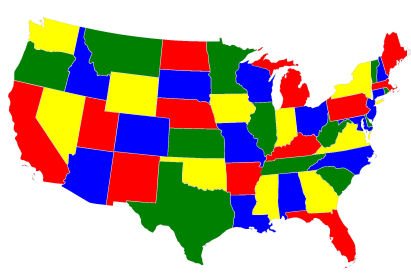
Fig. 33 Coloring a map of the USA.#
The Map Coloring: Complex Constraints advanced example demonstrates lower-level coding of a similar problem, which gives the user more control over the solution procedure but requires the knowledge of some system parameters (e.g., knowing the maximum number of supported variables for the problem). The Big Random Graph: dwave-hybrid Workflow example demonstrates the hybrid approach to problem solving in more detail by explicitly configuring the classical and quantum workflows.
Example Requirements#
The code in this example requires that your development environment have Ocean software and be configured to access SAPI, as described in the Configuring Access to the Leap Service (Basic) section.
Solution Steps#
Basic Workflow: Models and Sampling describes the problem-solving workflow as consisting of two main steps: (1) Formulate the problem as an objective function in a supported model and (2) Solve your model with a D‑Wave solver.
In this example, a function in Ocean software handles both steps. Our task is mainly to select the sampler used to solve the problem.
Formulate the Problem#
This example uses the NetworkX
read_adjlist() function to read a text file,
usa.adj, containing the states of the USA and their adjacencies (states with
a shared border) into a graph. The original map information was found on
write-only blog of Gregg Lind and looks like this:
# Author Gregg Lind
# License:  Public Domain.    I would love to hear about any projects you use if it for though!
#
AK,HI
AL,MS,TN,GA,FL
AR,MO,TN,MS,LA,TX,OK
AZ,CA,NV,UT,CO,NM
CA,OR,NV,AZ
CO,WY,NE,KS,OK,NM,AZ,UT

# Snipped here for brevity
You can see in the first non-comment line that the state of Alaska (“AK”) has Hawaii (“HI”) as an adjacency and that Alabama (“AL”) shares borders with four states.
>>> import networkx as nx
>>> G = nx.read_adjlist('usa.adj', delimiter = ',')
Graph G now represents states as vertices and each state’s neighbors as shared edges.
Solve the Problem by Sampling#
Ocean’s dimod can return a
minimum vertex coloring for a
graph, which assigns a color to the vertices of a graph in a way that no
adjacent vertices have the same color, using the minimum number of colors. Given
a graph representing a map and a sampler, the
min_vertex_coloring() function tries
to solve the map-coloring problem.
The dwave-hybrid package’s
KerberosSampler is classical-quantum hybrid
asynchronous decomposition sampler, which can decompose large problems into
smaller pieces that it can run both classically (on your local machine) and on
the D‑Wave quantum computer. Kerberos finds best samples by running in
parallel TabuProblemSampler,
SimulatedAnnealingProblemSampler, and D‑Wave
subproblem sampling on problem variables that have high impact. The only
optional parameters set here are a maximum number of iterations and number of
iterations with no improvement that terminates sampling. (See the
Big Random Graph: dwave-hybrid Workflow example for more details on
configuring the classical and quantum workflows.)
>>> import dwave.graphs
>>> from hybrid.reference.kerberos import KerberosSampler
>>> coloring = dwave.graphs.min_vertex_coloring(G, sampler=KerberosSampler(), chromatic_ub=4, max_iter=10, convergence=3)
>>> set(coloring.values())
{0, 1, 2, 3}
Note
The next code requires Matplotlib.
Plot the solution, if valid.
>>> import matplotlib.pyplot as plt
>>> node_colors = [coloring.get(node) for node in G.nodes()]
# Adjust the next line if using a different map
>>> if dwave.graphs.is_vertex_coloring(G, coloring):
...    nx.draw(G, pos=nx.shell_layout(G, nlist = [list(G.nodes)[x:x+10] for x in range(0, 50, 10)] + [[list(G.nodes)[50]]]), with_labels=True, node_color=node_colors, node_size=400, cmap=plt.cm.rainbow)
>>> plt.show()
The graphic below shows the result of one such run.
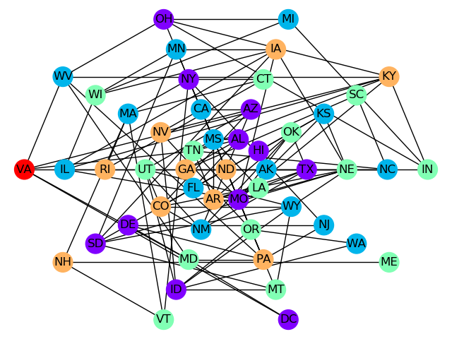
Fig. 34 One solution found for the USA map-coloring problem.#