Experimental Research

Some QPU solvers support experimental features used for advanced research. This section describes the currently supported features.

Note

Not all accounts have access to such research quantum computers.

Fast Reverse Annealing

Fast reverse annealing is an experimental feature to support limited use of the standard reverse annealing feature in the coherent regime of the quantum processing unit (QPU).

The generally available (GA) fast-anneal protocol enables sub-nanosecond annealing times, providing access to the QPU’s coherent regime. It does so by linearly ramping up the flux applied to the qubits, \(\Phi_{\rm CCJJ}\), in contrast to the slower standard-anneal protocol of linearly growing the qubits’ persistent current, \(I_p(s)\). This experimental feature, fast reverse annealing, enables reverse annealing in the coherent regime by rapidly ramping down \(\Phi_{\rm CCJJ}\). To maximize speed (the slope of the ramp), the QPU is programmed with an anneal schedule designed to overshoot the target normalized control bias, \(c(s)\).[1] Although the QPU cannot in fact follow this nominal annealing schedule, it achieves in this way reverse annealing in the coherent regime.

[1]

The normalized control bias is given by

\[c(s) = \frac{\Phi_{\rm CCJJ}(s) -\Phi_{\rm CCJJ}^{\rm initial}} {\Phi_{\rm CCJJ}^{\rm final} - \Phi_{\rm CCJJ}^{\rm initial}},\]

where \(\Phi_{\rm CCJJ}^{\rm initial}\) and \(\Phi_{\rm CCJJ}^{\rm final}\) are the values of \(\Phi_{\rm CCJJ}\) at \(s = 0\) and \(s = 1\), respectively (\(c(0) = 0\) and \(c(1)\) = 1).

Current Limitations

As noted above, in the current implementation, the QPU does not precisely follow anneal schedules set by the user. Consequently, some predefined schedules have been calibrated for use and the feature has the following restrictions.

• Where the standard reverse annealing supports a schedule of max_anneal_schedule_points points you can customize, which represents the QPU annealing with high accuracy, fast reverse annealing is restricted to a class of nominal schedules with a single shape: \(c(s)\) ramps down fast from the initial value \(c(s)=1\) to a value you select, pauses there for a duration you select, and then ramps back up fast to the final value \(c(s)=1\); this nominal schedule represents the QPU annealing only very loosely (Figure 136 and Figure 137 are more realistic depictions of the QPU annealing schedule).

• Durations of the pause can only be selected from a discrete set of supported values.

• The anneal_schedule must be provided although the configured values do not affect the executed schedule.

Usage

To submit a fast-reverse-annealing problem to the QPU, set the experimental x_target_c and x_nominal_pause_time parameters. Use the dwave-experimental get_parameters() function (you can also directly use the x_get_fast_reverse_anneal_exp_feature_info parameter) to view supported values for the feature parameters.

To assess for your nominal schedule (your configured target \(c(s)\) and pause duration), the anneal schedule that is executed by the QPU, use the utilities that the dwave-experimental repository provides, which can generate such graphs as those shown in Figure 136 and Figure 137. These figures show approximate schedules on the QPU for target \(c(s)\) set to 0 and 0.6 with various pause times.

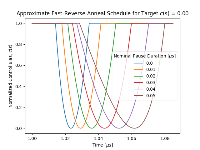
Fig. 136 Approximate fast-reverse-annealing schedule, showing the normalized control bias, \(c(s)\), as a function of time, with various pause durations, for a target \(c(s)=0\).

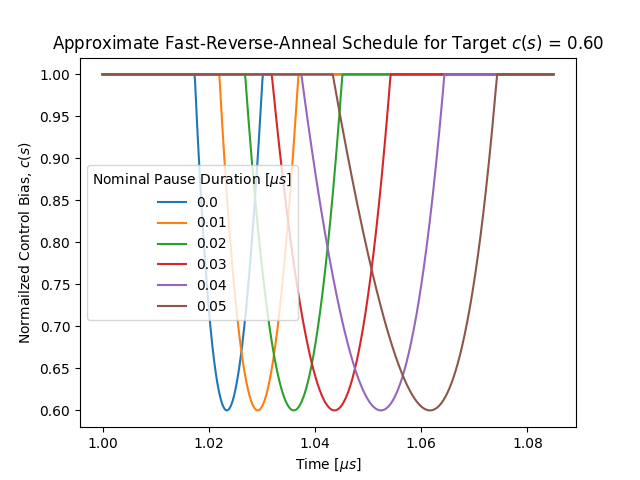
Fig. 137 Approximate fast-reverse-annealing schedule, showing the normalized normalized control bias, \(c(s)\), as a function of time, with various pause durations, for a target \(c(s)=0.6\).

Example: Larmor Precession

This example demonstrates Larmor Precession in a ring of qubits with ferromagnetic (FM) coupling. When subjected to fast reverse annealing, the measured populations of all-up and all-down spin states oscillate as expected.

The code below assumes that the following packages are installed: dwave-ocean-sdk (not all its packages are required), dwave-experimental, numpy, and tqdm (graphic progress meter, optional).

Accessing the QPU

To run the code on a QPU that supports this experimental feature and that your account has access to, ensure the following:

1. Set up your development environment as described in the Get Started with Ocean Software documentation.

2. Replace the placeholder name below with the solver name of your research node.

You can select a QPU and verify the selection as follows.

>>> from dwave.system import DWaveSampler
...
>>> qpu = DWaveSampler(solver="Advantage2_research1.4")
>>> print(qpu.solver.name)
Advantage2_research1.4

Embed the FM Ring

Create a FM ring of four qubits and find a minor-embedding. A four-qubit ring can be embedded with chain length of 1, as shown in this example’s output.

import dimod
from minorminer.subgraph import find_subgraph

num_qubits = 4   # Length of the FM ring
edges = [(i, (i + 1) % num_qubits) for i in range(num_qubits)]
embedding = find_subgraph(edges, qpu.edgelist)
bqm = dimod.BQM.from_ising(
    h={q: 0 for q in embedding.values()},  # For fast annealing, linear coefficients must be zero
    J={(embedding[v1], embedding[v2]): -1 for v1, v2 in edges})  # FM (J = -1) coupling

>>> print(embedding)
{0: 718, 1: 719, 2: 552, 3: 713}

Calibration Refinement

D-Wave provides a shimming tutorial that explains the need and methods for a more refined calibration used in such experiments as this one.

Flux-bias shimming is used here to calibrate qubits constituting the FM ring by centring the spin-up/spin-down oscillations around the expected ratio of 0.5 population value.

A simple calibration routine is to initialize the ring’s qubits in an all-up state, and for a range of target \(c(s)\) values, run a single fast reverse annealing and evaluate the populations of all-up and all-down states. The shim-learning rate is adaptively updated on each iteration using the hypergradient-descent method proposed in Online Learning Rate Adaptation with Hypergradient Descent by Atilim Gunes Baydin et al.

For more complex experiments, you can develop more sophisticated calibration techniques. The team at D-Wave will appreciate any techniques you wish to contribute to its Ocean software.

import numpy as np
from dwave.experimental.shimming import shim_flux_biases, qubit_freezeout_alpha_phi

sampler_params = dict(
    num_reads = 1024,
    answer_mode = "raw",
    reinitialize_state = True,
    initial_state = {q: 1 for q in embedding.values()},
    x_target_c = 0.25,
    x_nominal_pause_time = 0.0,
    anneal_schedule = [[0, 1], [1, 1]],     # Not used but currently required
    auto_scale = False,
    label="Fast Reverse Anneal: Calibration Refinement")

bqm_shim = dimod.BQM.from_ising(
    h = {q: 0 for q in embedding.values()}, # For fast annealing linear coefficients must be zero
    J = {(embedding[v1], embedding[v2]): 0 for v1, v2 in edges}) # No coupling for shim

x_target_c_updates = np.arange(0.2, 0.22, 0.001)

flux_biases, _, _ = shim_flux_biases(
    bqm=bqm_shim,
    sampler=qpu,
    sampling_params=sampler_params,
    sampling_params_updates = [{"x_target_c": x_target_c} for x_target_c in x_target_c_updates],
    symmetrize_experiments=False,
    learning_schedule=None,
    beta_hypergradient=0.4,
    alpha=0.1*qubit_freezeout_alpha_phi())

If you plot the values of the flux bias over the course of shimming, you should see convergence, as shown in Figure 138. This figure also shows how the flux-bias shimming minimizes the single-qubit magnetization averaged over the set of target \(c(s)\) values sampled on each iteration.

Fig. 138 Refinement of the flux-bias-offset calibration.

Run the Experiment

The code below runs the experiment.

from tqdm import tqdm

c_target_range = np.arange(0.2, 0.4, 0.0005)
num_samples = sampler_params['num_reads'] * num_qubits
sampler_params["label"] = "Fast Reverse Anneal: Larmor Experiment"

pro_up = []
pro_down = []
for target_c in tqdm(c_target_range):

    sampler_params['x_target_c'] = target_c

    sampleset = qpu.sample(bqm, flux_biases=flux_biases, **sampler_params)

    p_all_up = np.count_nonzero(sampleset.record.sample == 1)/num_samples
    p_all_down = np.count_nonzero(sampleset.record.sample == -1)/num_samples
    pro_up.append(p_all_up)
    pro_down.append(p_all_down)

Results should look similar to those shown in Figure 139.

Fig. 139 Measured populations of all-up versus all-down spin state showing an oscillating pattern as function of target \(c(s)\) as a result of Larmor precession.

Optional Graphic Code

The following code can be used to visualize results. The code requires that matplotlib is installed.

To view the refinement of the flux-bias-offset calibration, you can use the code below to plot outputs flux_biases, flux_bias_history, mag_history of the shim_flux_biases() function used above.

import matplotlib.pyplot as plt

mag_array = np.array(list(mag_history.values()))
flux_array = np.array(list(flux_bias_history.values()))
num_qubits = bqm_shim.num_variables
mag_array = np.reshape(mag_array, (num_qubits, 10, len(x_target_c_updates)))

plt.figure('all_fluxes')
plt.plot(flux_array.T)
plt.title("Calibration Results 1")
plt.xlabel("Shim Iteration")
plt.ylabel("Flux-Bias Offset ($\\Phi_0$)")
plt.legend(embedding.values(), title="Qubit Index")
plt.show()

plt.figure('all_avg_mags')
plt.title('Calibration Results 2')
for i in range(num_qubits):
    plt.plot(np.mean(mag_array, axis=2)[i])
plt.xlabel("Shim Iteration")
plt.ylabel("Averaged Single-Qubit Magnetization (a.u.)")
plt.legend(bqm.variables, title="Qubit Index")
plt.show()

To view the experiment results, you can use code such as the following.

plt.plot(c_target_range, pro_up, label='All Up')
plt.plot(c_target_range, pro_down, label='All Down')
plt.xlabel("Normalized Anneal Schedule $s$")
plt.ylabel("Spin Population")
plt.legend()
plt.title("Experiment Results")
plt.grid(True)
plt.show()

Multicolor Annealing

Multicolor annealing is an experimental feature to enable the programming of multiple anneal schedules for subsets of qubits on the quantum processing unit (QPU).

The generally available (GA) anneal_schedule parameter enables users to make changes to the global anneal schedule by submitting a set of points that define the piece-wise linear (PWL) waveform of the wanted annealing pattern. For example, you can change the standard schedule by introducing a pause or a quench, or you can initialize the qubits into a specific classical state and reverse anneal from there.

This experimental feature, multicolor annealing, lets you set a different anneal schedule for each of several subsets of qubits. You can also configure a schedule for large positive or negative polarizing flux biases to each subset of qubits.

Figure 140 shows the subsets of the QPU’s qubits on each of the six annealing lines of a particular Advantage2™ QPU with a Zephyr \(Z_6\) topology.

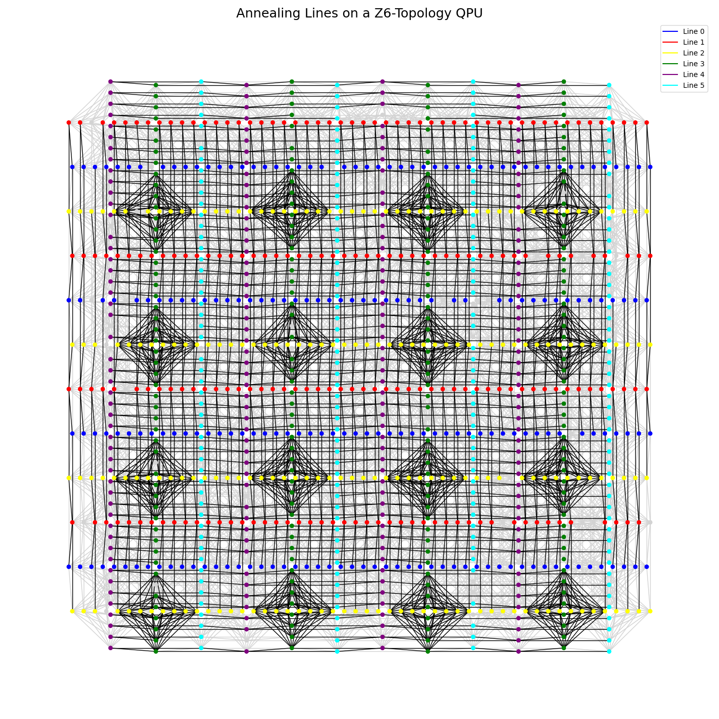
Fig. 140 A QPU with a \(Z_6\) topology shown with its six annealing lines in different colors.

Current Limitations

• Current implementation requires that the last points of anneal schedules set through the x_anneal_schedules must not be specified to a precision greater than the value of the minPolarizingTimeStep field.

• In the current implementation, you can specify the x_anneal_schedules parameter with a maximum precision of \(0.01\ \text{µs}\) (\(10\ \text{ns}\)). However, the x_schedule_delays parameter enables you to shift anneal schedules relative to each other with higher precision (\(1\ \text{ps}\)).

• Values of the normalized control bias, \(c(s)\), that extend beyond those corresponding to the highest and lowest possible transverse (tunneling) energy, \(A(c)\), are allowed only for a duration of \(0.02\ \text{µs}\). (You may do so to increase the generated waveform’s rate of change; see the x_get_multicolor_annealing_exp_feature_info section.)

• Scheduled flux biases applied to the qubits of an annealing line are limited to one very high or low value (polarization), and to zero (no polarization), in contrast to a range of flux biases that can be statically applied through the flux_biases parameter.

• For 2 microseconds after changing the polarization value from \(\pm 1\) to \(0\) for the qubits of an annealing line, you must not set a new value of the normalized control bias, \(c(s)\), through the x_anneal_schedules parameter, on that same line. This ensures that the flux biases are applying the expected offset value when the normalized control bias is changed on the polarized qubits.

• The range of values supported for the x_schedule_delays parameter, \([-100, 100]\) is not available in the information provided by the x_get_multicolor_annealing_exp_feature_info property.

• There may be an issue with specifying schedules to an overly high precision; if your solver returns an error that Time points must be quantized...., try rounding down your schedules:

  polarization_schedules[:, :, 0] = np.round(polarization_schedules[:, :, 0], 2)
  

Usage

Use the dwave-experimental get_properties() function (you can also directly use the x_get_multicolor_annealing_exp_feature_info property) to view supported values for the feature parameters.

To submit a multicolor-annealing problem to the QPU, set the following experimental parameters:

• x_anneal_schedules: Sets the anneal schedule for each subset of qubits.

• x_polarizing_schedules: Sets the schedule for flux biases to polarize each subset of qubits.

• x_disable_filtering: Disables software filtering of waveforms to match channel bandwidth, allowing faster anneal schedules.

• x_schedule_delays: Sets delays between the application of the anneal schedule of an annealing line relative to the others, enabling shifts with higher precision than the x_anneal_schedules parameter alone allows for.

Example: Larmor Precession In an Excited Qubit

This example demonstrates Larmor Precession of a target qubit after being diabatically excited into a superposition state by a coupled source qubit that undergoes reverse annealing from a state previously set by the application of a flux bias. This rapid reverse anneal of the source qubit causes a fast flux pulse into the target qubit, which has been annealed to some chosen extent where it was held. A detector qubit, also coupled to the target qubit, measures the spin state of the target qubit oscillating at a frequency determined by the energy barrier of the target qubit’s double-well potential, at the selected point in its anneal. Figure 141 illustrates the experimental setup.

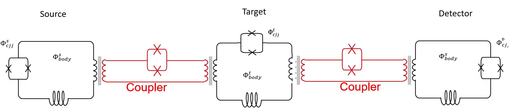
Fig. 141 Three coupled superconducting qubits used in the described experiment.

Figure 142 shows the energy landscape of each of the three qubits in this experiment, over time. The experiment starts by polarizing the source qubit with a flux-bias waveform while annealing it to a high value of the normalized control bias, \(c(s)\). Consequently, even when the polarizing waveform turns off, the high energy barrier keeps the source qubit locked in the state set by the polarizing bias. Next, the target qubit is annealed to a value of \(c(s)\), target_c, corresponding to some selected transverse energy, \(A(c)\), to which you wish to raise the energy barrier.[2]

The target qubit is biased by the state of the source qubit due to the coupling between them. Next, the source qubit is reverse annealed fast, lowering its energy barrier and removing the bias it applies to the target qubit, leaving the target qubit in an excited state. After a short but controlled delay (provided here by scanning the x_schedule_delays parameter), the detector qubit is quenched. This enables you to measure the spin state of the target qubit at short times after it is excited.

[2]

You can find the anneal schedules in the Per-QPU Solver Properties and Schedules section. Use the values provided for the fast-anneal protocol.

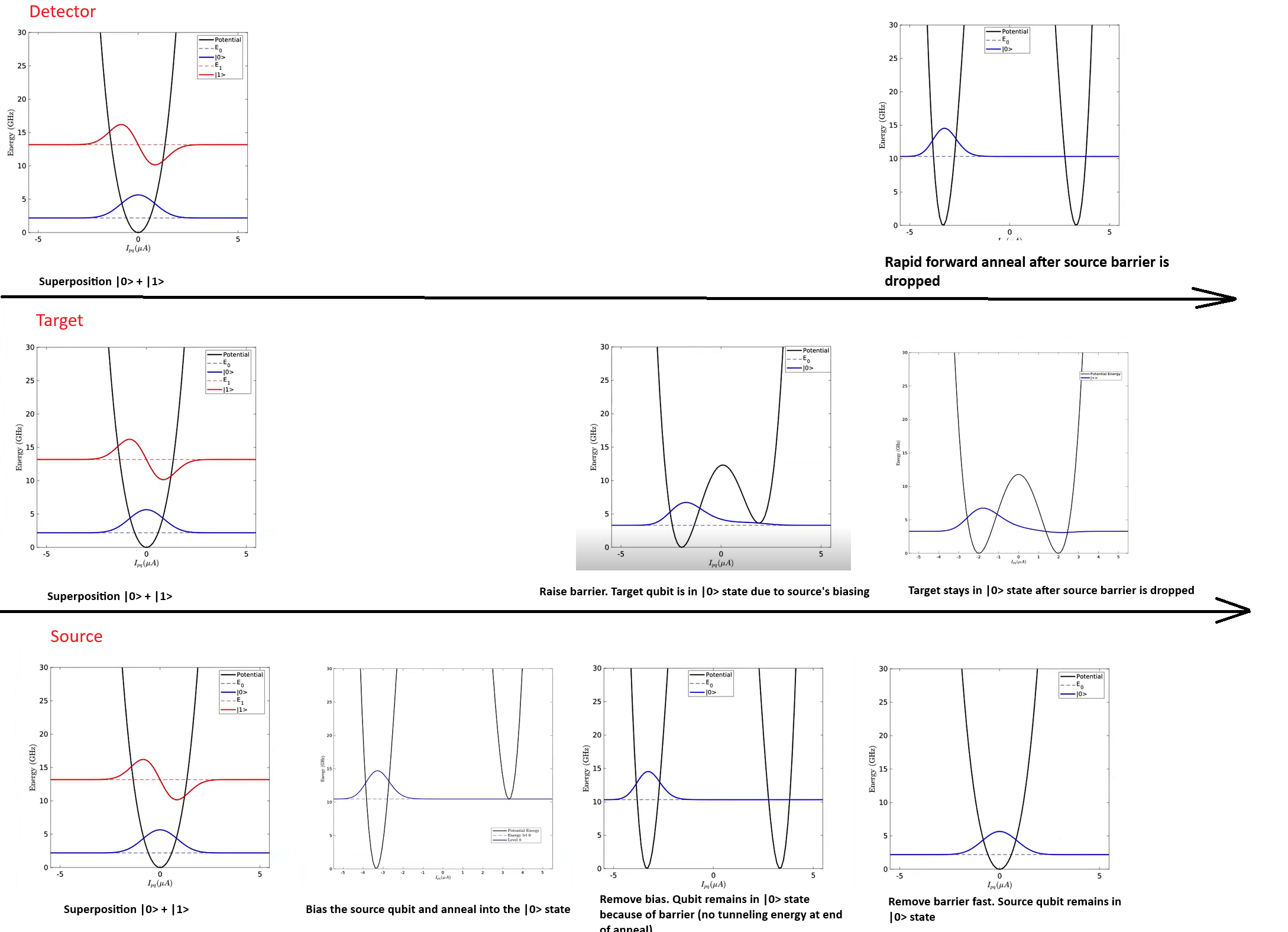
Fig. 142 Qubit potentials for each stage of the experiment.

The code below assumes that the following packages are installed: dwave-ocean-sdk (not all its packages are required), dwave-experimental, numpy, and tqdm (graphic progress meter, optional).

Accessing the QPU

To run the code on a QPU that supports this experimental feature and that your account has access to, ensure the following:

1. Set up your development environment as described in the Get Started with Ocean Software documentation.

2. Replace the placeholder name below with the solver name of your research node.

You can select a QPU and verify the selection as follows.

>>> from dwave.system import DWaveSampler, FixedEmbeddingComposite
...
>>> qpu = DWaveSampler(solver="Advantage2_research1.4")
>>> print(qpu.solver.name)
Advantage2_research1.4

Obtain Multicolor-Anneal Information

The x_get_multicolor_annealing_exp_feature_info property (in fact a parameter that functions in place of a property) returns information about per-line anneal schedules, such as the subset of the QPU’s qubits indexed to each line, supported minimum time steps, and ranges of normalized control bias, \(c(s)\), etc. Use this property to retrieve the information needed to use multicolor annealing on your selected QPU, either through the dwave-experimental get_properties() function (recommended) or directly.

1. Use the get_properties() function (recommended)

from dwave.experimental import multicolor_anneal as mca

exp_feature_info = mca.get_properties(qpu)

num_anneal_lines = len(exp_feature_info)

>>> print(f"QPU {qpu.solver.name} has {num_anneal_lines} annealing lines.")
QPU Advantage2_research1.4 has 6 annealing lines.

2. Alternatively, use the x_get_multicolor_annealing_exp_feature_info property directly.

computation = qpu.solver.sample_ising({qpu.nodelist[0]:0},
                                  {},
                                  num_reads=1,
                                  x_get_multicolor_annealing_exp_feature_info=True)

result = computation.result()
exp_feature_info = result['x_get_multicolor_annealing_exp_feature_info']

num_anneal_lines = len(exp_feature_info)

>>> print(f"QPU {qpu.solver.name} has {num_anneal_lines} annealing lines.")
QPU Advantage2_research1.4 has 6 annealing lines.

Embed the Experiment Qubits

The code below selects a random qubit on annealing line 0, to function in the experiment as the source of an excitation, and then finds a qubit on line 1 that is coupled to the first, which functions in the experiment as the target qubit, and finally finds a qubit on line 2 that is coupled to the target qubit, and serves as the detector qubit to make the measurements.

This method of embedding is pedagogic; for actual experiments it is recommended that you always embed logical problems as multiple embedded instances tiled across the full set of the QPU’s physical qubits in order to make best use of the system.

See the multicolor annealing example in the dwave-experimental repository.

import random

qubits_of_line = {}

for q in range(num_anneal_lines):
    qubits_of_line[q] = exp_feature_info[q]['qubits']

line_target = 0
line_source = 1
line_detector = 2

random_qubit_index = len(qubits_of_line[line_target])//2 + random.randrange(20)
Q_target = qubits_of_line[line_target][random_qubit_index]
adjacent = qpu.adjacency[Q_target]

attempts  = 2
while (
    attempts < 20 and
    not set(qubits_of_line[line_source]).intersection(set(adjacent)) and
    not set(qubits_of_line[line_detector]).intersection(set(adjacent))):

    print(f"Trying again ({attempts})")
    random_qubit_index = len(qubits_of_line[line_target])//2 + random.randrange(20)
    Q_target = qubits_of_line[line_target][random_qubit_index]
    adjacent = qpu.adjacency[Q_target]

    attempts += 1

Q_source= list(set(qubits_of_line[line_source]).intersection(set(adjacent)))[0]
Q_detector= list(set(qubits_of_line[line_detector]).intersection(set(adjacent)))[0]

embedding = {'Q_target': [Q_target], 'Q_source': [Q_source], 'Q_detector': [Q_detector]}
sampler = FixedEmbeddingComposite(qpu, embedding=embedding)

>>> print(f"""
... Target qubit {Q_target} on line {line_target}\nSource qubit {Q_source}
... on line {line_source}\nDetector qubit {Q_detector} on line {line_detector}
... """)
Target qubit 365 on line 0
Source qubit 370 on line 1
Detector qubit 371 on line 2

Calibration Refinement

D-Wave provides a shimming tutorial that explains the need and methods for a more refined calibration used in such experiments as this one.

See the dwave-experimental repository for refining calibration of the qubits. This pedagogic example does not refine calibration.

For more complex experiments, you can develop more sophisticated calibration techniques. The team at D-Wave will appreciate any techniques you wish to contribute to its Ocean software.

Obtain Boundary Values

Next, retrieve the maximum and minimum values you can use in creating an anneal schedule for the selected QPU.

Q_target_max_c = exp_feature_info[line_target]['maxC']
Q_target_min_c = exp_feature_info[line_target]['minC']

Q_source_max_c = exp_feature_info[line_source]['maxC']
Q_source_min_c = exp_feature_info[line_source]['minC']

Q_detector_max_c = exp_feature_info[line_detector]['maxC']
Q_detector_min_c = exp_feature_info[line_detector]['minC']

min_time_step = exp_feature_info[0]["minAnnealingTimeStep"]

>>> print(f"Minimum time step is {min_time_step} µs")
Minimum time step is 0.01 µs

Set Schedules

Next, set schedules for polarizing the source qubit, initializing the target qubit, exciting the target qubit with the source, and measuring the target qubit’s state by quenching the detector qubit.

1. Polarize the source qubit.

2. Anneal the source qubit to a high value of normalized control bias, \(c(s)\), raising its energy barrier.

3. Remove the polarizing bias on the source qubit. Because of the high energy barrier, the source qubit remains locked in the state set by the polarization.

4. Anneal the target qubit to target_c, a value of \(c(s)\) calculated for your chosen transverse energy, \(A(c)\), to which to raise the energy barrier. The target qubit is biased to the same state as the source qubit due to the antiferromagnetic coupling between them.

5. Reverse anneal the source qubit fast, lowering its energy barrier and removing the bias it applies to the target qubit, leaving the target qubit precessing in an excited state.

6. After a short but controlled delay (provided here by scanning the x_schedule_delays parameter), quench the detector qubit to measure the the spin state of the target qubit at short times after it is excited.

Figure 143 shows these schedules.

import numpy as np

target_c = 0.37

anneal_schedules = np.zeros((6, 8, 2))
anneal_schedules[line_source] = [
    [0.0, 0.0],[1.0, Q_source_max_c], [2.0, Q_source_max_c], [3.0, Q_source_max_c],
    [4.0, Q_source_max_c], [4.0 + min_time_step, Q_source_min_c],
    [5.0, Q_source_min_c], [6.0, 1.0]]

# Set supported time increments that can serve any non-participating annealing lines
anneal_schedules[:, :, 0] = anneal_schedules[line_source][:, 0]

anneal_schedules[line_target] = [
    [0.0, 0.0],[1.0, 0.0], [2.0, 0.0], [3.0, target_c],[4.0, target_c],
    [4.0 + min_time_step, target_c],[5.0, target_c], [6.0, 1.0]]

anneal_schedules[line_detector] = [
    [0.0, 0.0],[1.0, Q_detector_min_c], [2.0, Q_detector_min_c],
    [3.0, Q_detector_min_c], [4.0, Q_detector_min_c],
    [4.0 + min_time_step, Q_detector_max_c],[5.0, Q_detector_max_c], [6.0, 1.0]]

# Set supported time increments for any non-participating lines
polarization_schedules = np.zeros((6, 8, 2))
polarization_schedules[:, :, 0] = np.linspace(
    0.0, anneal_schedules[0][-1][0], anneal_schedules.shape[1])

polarization_schedules[line_source] = [
    [0.0, 1],[1.0, 1], [2.0, 0], [3.0, 0], [4.0, 0],
    [4.5, 0], [5.0, 0], [6.0, 0]]

You can visually validate your schedules by plotting them as shown in Figure 143.

Fig. 143 Anneal and polarization schedules for three qubits.

Run the Experiment

The code below runs the experiment. The three anneal and one polarization schedules, shown in Figure 143, are applied to each submission, with the delay between the target qubit’s reverse anneal and the detector qubit’s quench swept across a range of time values, delay_sweep, in the code. Figure 144 plots the spin population and shows a Larmor precession that corresponds to the chosen transverse energy, \(A(c)\), of the anneal for the target qubit.

from tqdm import tqdm
import dimod

qpu_parameters = dict(
    num_reads = 500,
    answer_mode = "raw",
    x_disable_filtering = True,
    x_schedule_delays = num_anneal_lines * [0.0],
    x_anneal_schedules = anneal_schedules,
    x_polarizing_schedules = polarization_schedules)

delay_sweep = np.arange(0.0, 0.02, 40*exp_feature_info[0]["scheduleDelayStep"])

res_plus=[]

for delay in tqdm(delay_sweep):
    qpu_parameters['x_schedule_delays'][line_detector] = delay
    sampleset = sampler.sample_ising(
        {},
        {('Q_target', 'Q_source'): -1, ('Q_target', 'Q_detector'): -1},
        **qpu_parameters,
        label="Multicolor Anneal: 3Q Lamar Precession Experiment")
    sample = dimod.keep_variables(sampleset, ['Q_detector']).record.sample
    res_plus.append(np.mean(sample))

Results should look similar to those of Figure 144.

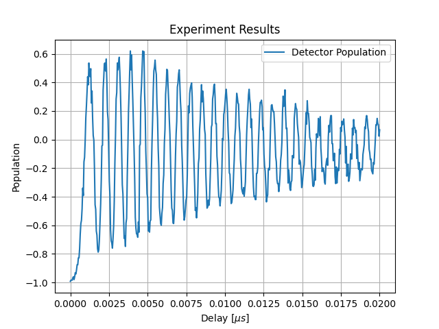
Fig. 144 Experiment results showing Larmor precession.

Optional Graphic Code

The following code can be used to visualize results. The code requires that matplotlib is installed.

To view schedules, you can use code such as the following.

import matplotlib.pyplot as plt

def plot_anneal_3q(anneal_pwl, fb_pwl, title):

    anneal = np.asarray(anneal_pwl)
    fb = np.asarray(fb_pwl)

    fig, ax = plt.subplots(3, 1, figsize=(10, 5))

    for indx, line in enumerate([line_source, line_target, line_detector]):

        ax[indx].plot(anneal[line][:,0], anneal[line][:,1], 'blue', label="Anneal")

        ax[indx].set_title(title[indx])

        ax_twin = ax[indx].twinx()
        ax_twin.plot(fb[line][:,0], fb[line][:,1], 'orange', label="Flux Bias")
        ax[indx].grid(axis='both', linestyle='--')

    ax[2].set_xlabel('Time $\\mu s$')
    ax[1].set_ylabel('Normalized Control Bias $c(s)$', color='blue')
    ax_twin = ax[1].twinx()
    ax_twin.set_ylabel('Flux-Bias Offset', color='orange', labelpad=20)
    plt.subplots_adjust(hspace=0.6)
    plt.tight_layout()

To view the experiment results, you can use code such as the following.

plt.plot(delay_sweep, res_plus, '.-', label='Spin Population')
plt.xlabel("Delay [$\mu s$]")
plt.ylabel("Spin Population")
plt.legend()
plt.grid(True)
plt.title("Experiment Results")
plt.show()

dwave-experimental Utilities

The dwave-experimental repository provides Ocean utilities to support advanced QPU prototype features. It also contains useful code examples.

SOLVER_FILTER = {'name__regex': 'Advantage2_prototype2.*|Advantage2_research1\\..*'}

Filter for an available solver that supports advanced annealing features.

Feature-based solver selection returns the first available solver that supports features such as fast reverse annealing.

Note

currently SAPI does not support filtering for solvers with experimental research features, so a simple pattern matching is used.

Example::

>>> from dwave.system import DWaveSampler
>>> from dwave.experimental import fast_reverse_anneal as fra
...
>>> with DWaveSampler(solver=fra.SOLVER_FILTER) as sampler:
        sampler.sample(...)

get_solver_name() → str

Return the name of a solver that supports advanced annealing features.

The result is memoized, so the API is queried only on first call.

Examples

>>> from dwave.experimental.fast_reverse_anneal import get_solver_name
...
>>> print(get_solver_name())
Advantage2_research1.4

Fast Reverse Annealing

get_parameters(sampler: DWaveSampler | StructuredSolver | str | None = None) → dict[str, Any]

Return available fast-reverse-annealing parameters and their information.

Parameters:

sampler – A DWaveSampler sampler that supports the fast-reverse-anneal (FRA) protocol. Alternatively, you can specify a StructuredSolver solver or a solver name. If unspecified, SOLVER_FILTER is used to fetch an FRA-enabled solver.

Returns:

Each parameter available is described with its data type, value limits, an is-required flag, a default value (if it’s optional), and a short description.

Examples

Use an instantiated DWaveSampler sampler:

>>> from dwave.system import DWaveSampler
>>> from dwave.experimental import fast_reverse_anneal as fra
...
>>> with DWaveSampler() as sampler:
...    param_info = fra.get_parameters(sampler)

c_vs_t(t: numpy.typing.ArrayLike, *, target_c: float, nominal_pause_time: float = 0.0, upper_bound: float = 1.0, schedules: dict[str, float] | None = None) → numpy.typing.ArrayLike

Calculate the approximate normalized control bias.

Approximates the time-dependent normalized control bias \(c(s)\) using a linear-exponential function, linex(), for simulating fast-reverse-anneal waveforms.

Parameters:

• t – Discrete time, in microseconds, as a scalar or an array.

• target_c – The lowest value of the normalized control bias, \(c(s)\), reached during a fast reverse annealing.

• nominal_pause_time – Pause duration, in microseconds, for the fast-reverse-annealing schedule.

• upper_bound – Waveform’s upper bound.

• schedules – Schedule family parameters, as returned by the load_schedules() function.

Returns:

Schedule waveform approximation evaluated at t.

Examples

Obtain an estimated normalized control bias \(c(s)\), at time 0.022, for a waveform that reaches \(c(s)=0\) at its lowest point and nominally pauses there for 0.02 microsecond.

>>> from dwave.experimental import fast_reverse_anneal as fra
...
>>> c = fra.c_vs_t(0.022,
...     target_c=0.0,
...     nominal_pause_time=0.02,
...     schedules=fra.schedule.load_schedules())

linex(t: numpy.typing.ArrayLike, *, c0: float, c2: float, a: float, t_min: float) → numpy.typing.ArrayLike

Approximate the fast-reverse-annealing schedule at a given time.

Uses a linear-exponential (“linex”) function to approximate a fast-reverse-annealing schedule with the following linear-exponential function,

\(f(t) = c_0 + \frac{2 c_2}{a^2} \left(e^{a(t - t_{\min})} - a(t - t_{\min}) - 1\right)\),

where \(t\) is discrete time, in microseconds, \(c_0\) is an ordinate offset coefficient, \(c_2\) is a quadratic ordinate coefficient, \(a\) is an asymmetry parameter, and \(t_{\text{min}}\) is a time offset parameter.

Parameters:

• t – Discrete time, in microseconds, as a scalar or an array.

• c0 – \(c_0\) is an ordinate offset coefficient.

• c2 – \(c_2\) is a quadratic ordinate coefficient.

• a – \(a\) is an asymmetry parameter.

• t_min – \(t_{\text{min}}\) is a time offset parameter.

Returns:

The linear-exponential function evaluated at t.

Examples

See source code of the c_vs_t() function for a usage example.

load_schedules(solver_name: str | None = None) → dict[float, dict[str, float]]

Return fast-reverse-annealing schedule-approximation parameters.

The approximation parameters are for all allowed values of pause duration, and used in the following formula,

\(f(t) = c_0 + \frac{2 c_2}{a^2} \left(e^{a(t - t_{\min})} - a(t - t_{\min}) - 1\right)\),

where \(t\) is discrete time, in microseconds, \(c_0\) is an ordinate offset coefficient, \(c_2\) is a quadratic ordinate coefficient, \(a\) is an asymmetry parameter, and \(t_{\text{min}}\) is a time offset parameter.

Parameters:

solver_name – Name of a QPU solver that supports fast reverse annealing. If unspecified, a call to SAPI is made to determine the default solver (a QPU that supports fast reverse annealing) .

Returns:

A dict mapping supported values of the x_nominal_pause_time parameter to dicts of parameters that can be used to approximate the (linear-exponential) annealing schedule of the QPU. For example:

{0.0: {'a': -51.04360118925347,
    'c2': 9821.41471886313,
    'nominal_pause_time': 0.0,
    't_min': 1.0234109310649393},
...}

Examples

Obtain the schedule-approximation parameters for the default solver that supports fast reverse annealing.

>>> from dwave.experimental import fast_reverse_anneal as fra
...
>>> param_002 = fra.schedule.load_schedules()[0.02]
>>> list(param_002.keys())
['nominal_pause_time', 'a', 'c2', 't_min']
>>> tmin_002 = param_002['t_min']

plot_schedule(t: numpy.typing.ArrayLike, *, target_c: float, nominal_pause_time: float = 0.0, schedules: dict[str, float] | None = None, figure: Figure | None = None) → Figure

Plot the approximate fast-reverse waveform.

Creates a plot of the approximate fast-reverse waveform for a given target_c and nominal_pause_time, using time grid t, optionally adding to an existing figure figure.

Example

>>> import numpy
>>> import matplotlib.pyplot as plt
>>> from dwave.experimental.fast_reverse_anneal import plot_schedule
...
>>> t = numpy.arange(1.0, 1.04, 1e-4)
>>> fig = plot_schedule(t, target_c=0.0)
>>> plt.show()

See also: examples directory.

Multicolor Annealing

get_properties(sampler: DWaveSampler | StructuredSolver | str | None = None) → list[dict[str, Any]]

Return multicolor-annealing properties for each annealing line.

Parameters:

sampler – A DWaveSampler sampler that supports the multicolor annealing (MCA) protocol. Alternatively, you can specify a StructuredSolver solver or a solver name. If unspecified, SOLVER_FILTER is used to fetch an MCA-enabled solver.

Returns:

Annealing-line properties for all available annealing lines, formatted as list of dicts in ascending order of annealing-line index.

Examples

Retrieve MCA properties for the annealing lines of a default solver, and print the number of lines and first qubits on line 0.

>>> from dwave.experimental import multicolor_anneal as mca
...
>>> annealing_lines = mca.get_properties()
>>> len(annealing_lines)
6
>>> annealing_lines[0]['qubits']
[2, 6, 9, 14, 17, 18, ...]

Shimming

qubit_freezeout_alpha_phi(eff_temp_phi: float = 0.112, flux_associated_variance: float = 0.0009765625, estimator_variance: float = 0.00390625, unit_conversion: float = 0.001148)

Determine the learning rate for independent qubits.

For a qubit offset by \(\Phi_{0i}\) that is to be corrected by a choice of flux bias \(\Phi\), a model of single-qubit freezeout dictates that magnetization \(<s_i> = tanh(\frac{\Phi_{0i} + \Phi_i}{T})\), where \(T\) is the effective temperature.

Assume the unshimmed magnetization to be zero-mean distributed with small variance, \(\Delta_1\), and a standard sampling-based estimator with variance \(\Delta_2 = \frac{1}{\text{num_reads}}\). You can then determine an update to the flux, \(\Phi = l <s_i>_{\text{data}}\), where the learning rate \(l = T \frac{\Delta_1}{Delta_1 + Delta_2}\). This update is optimal in the sense that it minimizes the expected square magnetization.

For correlated spin systems and/or experiments that are not well described by thermal freezeout, a data-driven approach is recommended to determining the schedule and related parameters. The freezeout (Boltzmann) distribution can be extended to correlated models, wherein the covariance matrix plays a role in determining the optimal learning rate. A single qubit rate can remain a good approximation given weakly correlated spins.

Parameters:

• eff_temp_phi – Effective (unitless) inverse temperature at freezeout. This can be determined from current device parameters.

• flux_associated_variance – The expected variance of the magnetization (\(m\)) due to flux offset.

• estimator_variance – The expected variance in the magnetization estimate, \(\frac{1-m^2}{\text{num_reads}}\).

• flux_scale – Conversion from units of h to units of \(\Phi\) can be determined from published device parameters. See h_to_fluxbias().

Returns:

An appropriate scale for the learning rate, minimizing the expected square magnetization.

Example

Determining an \(\alpha_\Phi\) appropriate for forward anneal of a weakly coupled system, Advantage_system4.1 based on published parameters. Note that defaults (by contrast) are determined based on published values for Advantage2_system1.3.

>>> from dwave.experimental.shimming import qubit_freezeout_alpha_phi
...
>>> alpha_phi = qubit_freezeout_alpha_phi(
...     eff_temp_phi=0.198,
...     flux_associated_variance=1/1024,
...     estimator_variance=1/256,
...     unit_conversion=1.647e-3)

shim_flux_biases(bqm: BinaryQuadraticModel, sampler: Sampler, *, sampling_params: dict[str, Any] | None = None, shimmed_variables: Iterable[Hashable] | None = None, learning_schedule: Iterable[float] | None = None, convergence_test: Callable | None = None, symmetrize_experiments: bool = True, sampling_params_updates: list | None = None, beta_hypergradient: float = 0.4, num_steps: int = 10, alpha: float | None = None) → tuple[list[float | floating | integer], dict, dict]

Return flux biases that minimize magnetization for symmetry-preserving experiments.

You can refine calibration for specific QPU experiments by modifying your QPU programming. The flux bias parameter compensates for low-frequency environmental spins that couple into qubits, distorting the target distribution. Although you can modify either flux bias or h to restore symmetry of the sampled distribution, flux biases more accurately eliminate common forms of low-frequency noise.

Assuming the magnetization (expectation for measured spins, or sign of the persistent current) is a smooth, monotonic function of the qubit body’s magnetic fluxes (flux bias), you can determine parameters that achieve a target magnetization, \(m\), by iterating \(\Phi(t+1) \leftarrow \Phi(t) - L(t) (<s> - m)\), where \(L(t)\) is an iteration-dependent map, \(<s>\) is the expected magnetization, \(m\) is the target magnetization, and \(\Phi\) are the programmed flux biases.

By default \(L(t)\) is uniform with respect to programmed qubits, and determined by a hypergradient descent method. Alternatively you can specify the learning rate as a list, in which case the hypergradient method is not used.

Symmetry can be broken by the choice of initial condition in reverse annealing, non-zero \(h\), x_polarizing_schedules, or non-zero flux biases over unshimmed fluxes. You can collect data for two experiments, with inverted symmetry breaking between them, anticipating zero magnetization in the experimental average rather than per experiment. Shimming based on this symmetrized data set is expected to determine a good shim for both experiments, assuming a weak dependence of noise on the symmetry-breaking field.

Where strong correlations, or strong symmetry-breaking effects, are present in an experiment, the sampled distribution may contain insufficient information to independently shim all degrees of freedom. Shims are expected to be a smooth function of annealing parameters such as annealing time, anneal schedule, and Hamiltonian parameters. You can use shims inferred in smoothly related models as approximations (or initial conditions) for searches in target models.

If the provided learning rate or learning schedule is too large, it is possible to exceed the bounds of allowed values for the flux-bias offsets.

Parameters:

• bqm – A BinaryQuadraticModel.

• sampler – A DWaveSampler.

• sampling_params – Parameters of the DWaveSampler. Note that if sampling_params contains flux biases, these are treated as an initial condition and edited in place. Chose a value for the num_reads parameter in conjunction with your chosen schedule. Note that, the initial_state parameter, if provided, is assumed to be specified according the Ising model convention (\(\pm 1\), and \(-3\) for inactive).

• shimmed_variables – A list of variables to shim; by default all elements in variables.

• learning_schedule – An iterable of gradient-descent prefactors. When not provided, prefactors are determined by a hypergradient-descent method parameterized by the alpha, beta_hypergradient, and num_steps arguments.

• convergence_test – A callable that take the history of magnetizations and flux biases as input, returning True to exit the search, and False otherwise. By default, all stages specified in the learning_schedule argument are completed.

• symmetrize_experiments – If True, performs a test to determine symmetry breaking in the experiment: a non-zero initial_state for reverse anneal, non-zero \(h\), or non-zero flux_biases (on some unshimmed variables). If any of these are present, magnetization is inferred by averaging over two experiments with symmetry-breaking elements inverted. The shim averages the symmetrically related experiments to achieve zero magnetization.

• sampling_params_updates –

  Where you require averaging across many experiments, you can specify a list of updates. Each element in your list is a dictionary that updates the sampling_params argument. Experiments are averaged over these sampling-parameter updates to determine the magnetization used in shimming. The original value of the updated sampling parameter is ignored. The flux_biases parameter must not be an updated parameter. See the examples directory for use cases.

• beta_hypergradient – Controls the learning rate evolution for the hypergradient-descent method, enabling improved performance through customizing for the annealing protocol and QPU. Supported values are in range \((0,1)\). Ignored if you specify the learning_schedule argument.

• num_steps – Number of steps taken by the hypergradient-descent method if you do not specify a learning_schedule from which to infer. Default is 10 if neither is specified.

• alpha – Initial learning rate for the hypergradient-descent method, enabling improved performance through customizing for the annealing protocol and QPU. Supported values are positive, real floats with a typical scale you can determine using the qubit_freezeout_alpha_phi() function. By default, initialized using the qubit_freezeout_alpha_phi() function. Ignored if you specify the learning_schedule argument.

Returns:

1. Flux biases in a list using the flux_biases format (for use by a DWaveSampler sampler).

2. History of flux-bias assignments per shimmed component.

3. History of magnetizations per shimmed component.

Return type:

A tuple consisting of 3 parts

Example

See the examples test directories for additional use cases.

Shim degenerate qubits at constant learning rate and solver defaults. The learning schedule and number of reads is for demonstration only, and has not been optimized.

>>> import numpy as np
>>> import dimod
>>> from dwave.system import DWaveSampler
>>> from dwave.experimental.shimming import shim_flux_biases, qubit_freezeout_alpha_phi
...
>>> qpu = DWaveSampler()
>>> bqm = dimod.BQM.from_ising({q: 0 for q in qpu.nodelist}, {})
>>> alpha_phi = qubit_freezeout_alpha_phi()  # Unoptimized to the experiment, for demonstration purposes.
>>> ls = [alpha_phi]*5
>>> sp = {'num_reads': 2048, 'auto_scale': False}
>>> fb, fb_history, mag_history = shim_flux_biases(bqm,
...     qpu,
...     sampling_params=sp,
...     learning_schedule=ls)
...
>>> print(f"RMS magnetization by iteration: {np.sqrt(np.mean([np.array(v)**2 for v in mag_history.values()], axis=0))}")