

Max Cut: QA Vs. LR-QAOA#
An IonQ paper, “Measuring what matters: A scalable framework for application-level quantum benchmarking” [Abo2026], uses linear-ramp quantum approximate optimization algorithm (LR-QAOA), a variational quantum algorithm, to solve maximum-cut problems on regular and fully-connected graphs on IonQ Forte-1. This vignette compares the results to those from quantum annealing on D-Wave’s Advantage2 system.
Problem Instances#
The max cut problem is to partition the vertices of a graph into two sets such that the number of edges (or the sum of the weights of the edges) between the two sets is maximized. The Hamiltonian can be expressed as:
where \(E(G)\) is the set of edges in the graph, \(w_{ij}\) is the weight of the edge between vertices \(i\) and \(j\), and \(s_i\) is a spin variable.
The problems are instances of max cut on regular graphs of degree 3 and 4 (cubic and quartic graphs) on 24 and 36 vertices and fully-connected graphs on 12 and 16 vertices, with one instance per class. The graphs and optimal solutions are given in the IonQ GitHub repository.
Methodology#
Since the problem graphs are relatively small compared to the size of the Advantage2 QPU, the graphs can be embedded multiple times into a single QPU and sampled from simultaneously. Therefore each read from the QPU is comprised of a number of samples equal to the number of embeddings. The best solution from each read is taken to compute the approximation ratio (AR) of that sample. Ocean software’s minorminer is used to find parallel minor embeddings of the problem graphs onto the Advantage2 QPU’s Zephyr topology. The number of embeddings found for each problem instance is given in the table below:
Graph Type |
Number of Embeddings |
|---|---|
Clique with n=12 |
113 |
Clique with n=16 |
66 |
3-regular graph with n=24 |
147 |
3-regular graph with n=36 |
94 |
4-regular graph with n=24 |
127 |
4-regular graph with n=36 |
71 |
For this study, embeddings were selected based on a maximum chain length of 4 and best average chain length out of 10.
The problems were run with the
ParallelEmbeddingComposite and
ScaleComposite composites with
extended J ranges on D-Wave’s
Advantage2_system1 QPU.
The following code shows an example of creating a binary quadratic model
(BQM) for a max-cut problem, embedding it multiple times into the QPU,
sampling from the QPU, and returning the SampleSet.
import networkx as nx
import dimod
from dwave.preprocessing.composites import ScaleComposite
from dwave.system import DWaveSampler, ParallelEmbeddingComposite
from minorminer import find_embedding

# create problem graph
G = nx.random_regular_graph(2, 10)

# create bqm for max cut on G
bqm = dimod.BinaryQuadraticModel(vartype = dimod.SPIN)

for u, v, g_data in G.edges(data = True):
    bqm.add_quadratic(int(u), int(v), g_data.get('weight', 1))

# find parallel minor embeddings of G into the QPU graph
qpu_sampler = DWaveSampler(solver='Advantage2_system1')
qpu_graph = qpu_sampler.to_networkx_graph()

parallel_embeddings = []

keep_embedding = True
while keep_embedding:
    embedding = find_embedding(G.edges, qpu_graph)
    if len(embedding) > 0:
        parallel_embeddings.append(embedding)
        qpu_graph.remove_nodes_from([node for val in embedding.values() for node in val])
    else:
        keep_embedding = False

# create sampler with parallel embeddings and scale composite
embedded_sampler = ParallelEmbeddingComposite(ScaleComposite(qpu_sampler), embeddings=parallel_embeddings)

# sample from the QPU
sampleset = embedded_sampler.sample(
    bqm,
    num_reads=5000//len(parallel_embeddings),
    annealing_time=20,
    quadratic_range=qpu_sampler.properties["extended_j_range"],
    bias_range=qpu_sampler.properties["h_range"],
    auto_scale=False
)
Results#
Time-to-Solution#
The computation of time per sample used for the results below follows the conventions from [Abo2026] and the Benchmarking Verification Report. Therefore, the time per shot is computed by taking the total runtime, subtracting some unspecified overhead time and dividing by the number of shots, which is 5,000. This gives a time per shot of 0.89 seconds for IonQ Forte-1. Since it is unclear how much overhead was removed, the time per sample for D-Wave’s Advantage2 system is taken to be the annealing time plus the readout time. For max cut on the 4-regular graph with 36 nodes and 20 \(\mu s\) annealing time, the time per sample is 118 \(\mu s\) for the Advantage2 QPU.
The approximation ratio (AR) of a solution is the energy of that solution divided by the energy of the optimal solution. Let \(p_s\) be the proportion of samples whose AR is greater than or equal to a designated lower bound (denoted AR_min). The time-to-solution (TTS) at 99% confidence for a specified value of AR_min is calculated as \(TTS = N_{shots}*t_{shot}\), where \(N_{shots} = \ln(0.01)/\ln(1-p_s)\). Note that in the proposed TTS formula, a probability of success above 99% results in \(N_{shots} < 1\), but a fraction of a shot is not possible. Therefore, the integer ceiling function is used to ensure shots are integers: \(N_{shots} = \lceil \ln(0.01)/\ln(1-p_s) \rceil\). Since more than 99% of the samples from D-Wave’s Advantage2 system are at or above all values of AR_min in the plot, this results in a TTS equal to the time per sample, 118 \(\mu s\).
The time-to-solution results are displayed in Figure 215. D-Wave’s Advantage2 system demonstrates a speedup of up to 7 orders of magnitude over IonQ Forte-1.
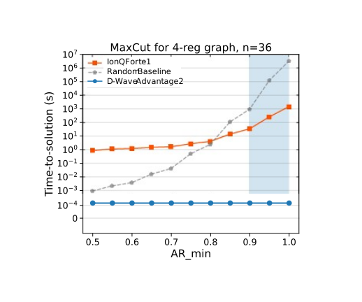
Fig. 215 D-Wave’s Advantage2 system demonstrates a speedup of up to 7 orders of magnitude over IonQ Forte-1. Also shown is the result of the random samples as described in the next section.#
Sample Distribution#
In the Benchmarking Verification Report, the estimated time per shot for IonQ Forte-1 is 0.89 s. For the max cut problem on the 4-regular graph with 36 nodes, the percentage of samples above 90% AR is approximately 10% for IonQ Forte-1. For the Advantage2 QPU with 20 \(\mu s\) annealing time and 118 \(\mu s\) per sample, the percentage of samples above 90% AR is 100%. In fact, when taking the best solution found for each sample of the parallel embeddings of the problem in the QPU, all have an AR of 100%, corresponding to the optimal solution.
The sample distributions shown in Figure 216 include all samples across all embeddings from D-Wave’s Advantage2 system.
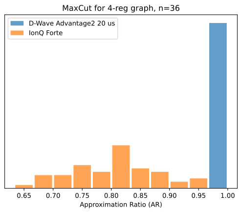
Fig. 216 Every sample from D-Wave’s Advantage2 system has a higher AR than all samples from IonQ Forte-1.#
Approximation Ratios and Time per Sample#
The table below shows the approximation ratios and time per sample for IonQ’s Aria-1 and Forte-1 systems and D-Wave’s Advantage2 system on all instances of 3- and 4-regular graphs and fully-connected weighted (FCW) graphs. The reported approximation ratio (AR) is the mean AR across all samples for a given problem instance. The effective approximation ratio (AR_eff) is the mean effective AR, which is the AR rescaled with respect to a random baseline (AR_rand), where \(AR_{rand} = \mu_{rand} + 3\sigma_{rand}/\sqrt{5,000}\). Here, \(\mu_{rand}\) and \(\sigma_{rand}\) are the mean and standard deviation of the ARs taken from 5,000 random samples.
In the original table from the paper, the values are purported to be effective AR, but some values appear to be regular AR based on the appearance of the plots. Using the calculated values of AR_rand, the missing values (whether AR or AR_eff) are estimated and added to the table. The values reported for D-Wave’s Advantage2 system are mean AR and AR_eff with 20 \(\mu s\) annealing time.
The results show that quantum annealing on D-Wave’s Advantage2 system finds a better mean approximation ratio for all problems and with much shorter sample times compared to LR-QAOA on IonQ’s Forte-1 and Aria-1 systems. All but one of the mean AR values for D-Wave’s Advantage2 system are 1, corresponding to the optimal solution.
Problem Instance |
IonQ Aria-1 AR (AR_eff) |
IonQ Forte-1 AR (AR_eff) |
IonQ Forte-1 Time per Sample (s) |
D-Wave Advantage2 AR (AR_eff) |
D-Wave Advantage2 Time per Sample (s) |
|---|---|---|---|---|---|
3-reg, n=24 |
– |
0.8390 (0.6123) |
– |
1.0 (1.0) |
1.18e-04 |
3-reg, n=36 |
– |
0.7841 (0.5280) |
– |
1.0 (1.0) |
1.18e-04 |
4-reg, n=24 |
– |
0.8668 (0.6365) |
– |
1.0 (1.0) |
1.18e-04 |
4-reg, n=36 |
– |
0.8009 (0.5197) |
0.89 |
1.0 (1.0) |
1.18e-04 |
FCW, n=12 |
0.8711 (0.3728) |
0.8669 (0.3821) |
– |
1.0 (1.0) |
1.22e-04 |
FCW, n=16 |
– |
0.8459 (0.2504) |
– |
0.995 (0.9757) |
1.15e-04 |