Satellite Placement#

In the satellite-placement problem, a set of satellites, each having east and west boundaries, is to be placed along an arc. Between each pair of satellites, there is interference that decreases with distance. The goal is to place the satellites so that the maximum interference experienced by any pair is minimized.

Problem Instances#

Global west and east boundaries are set to 0 and 180. Midpoints for each satellite’s range are generated uniformly in [0,180], and a radius of up to 70 (not going beyond 0 or 180) determines the range. Interferences are generated uniformly between 0 and 1. There are 11 problem instances for each number of satellites.

Mathematical Models#

Mixed Integer Programming (MIP) Formulation#

The MIP formulation is based on the formulation provided in [Spa1991] and is used by the CQM solver. The locations of the satellites are represented by continuous variables \(\theta_i\). Satellite orders are encoded by binary variables. An integer variable \(z\) is needed to help track the interferences experienced by each pair of satellites. Additional binary variables are needed to reduce the degree of the constraints, as the CQM solver can handle at most quadratic terms. These additional binary variables are set equal to the product of each pair of the original binary variables, meaning that the number of these variables is quartic in the number of satellites.

Mixed Integer Nonlinear Programming (MINLP) Formulation#

The Pyomo modeling language with IPOpt (Interior Point Optimization) can use absolute value rather than encoding the order of the satellites with binary variables. Here, \(z\) and \(\theta_i\) are continuous variables, \(d_{ij}\) is the interference between satellites \(i\) and \(j\), and \(W_i\) and \(E_i\) are the west and east boundaries of satellite \(i\). The formulation is then the same as in [Spa1991]:

\[\begin{split}\begin{array}\\ \text{maximize } &z\\ \text{such that } & d_{ij}z \leq |\theta_j -\theta_i| \leq 360-d_{ij}z & \forall 1 \leq i < j \leq n\\ &W_i \leq \theta_i \leq E_i & \forall 1 \leq i \leq n\\ \end{array}\end{split}\]

Nonlinear Solver Formulation#

This formulation makes use of a list() variable to eliminate the need for the binary variables in the MIP formulation encoding the order of the satellites. To introduce continuous variables in the model, the LinearProgram class is used.

For each satellite ordering, there is an associated linear program:

\[\begin{split}\begin{array}\\ \text{minimize } & c\mathbf{x}\\ \text{such that }& A\mathbf{x} \leq b\\ \text{and } & l \leq \mathbf{x} \leq u\\ \end{array}\end{split}\]

The linear program is determined by the inequalities below:

\[\begin{split}\begin{array}\\ \theta_j - \theta_i + d_{\sigma(i)\sigma(j)}z \leq 0\\ -\theta_j + \theta_i + d_{\sigma(i)\sigma(j)}z \leq 360\\ \end{array}\end{split}\]

Here, \(d_{\sigma(i)\sigma(j)}\) is the interference between the satellites in the \(i^{\text{th}}\) and \(j^{\text{th}}\) positions. The matrix \(A\) of the linear program is determined by the coefficients of the left-hand sides of the inequalities, and the vector \(\mathbf{b}\) is equal to \((0,\ldots,0,360,\ldots,360)\), determined by the right-hand sides.

The upper and lower bound vectors \(l\) and \(u\) are the west and east boundaries \(W_{\sigma(i)}\) and \(E_{\sigma(i)}\), ordered by the state of the list variable.

Finally, to maximize \(z\), define the vector \(\mathbf{c}\) to be \((0,\ldots,0,-1)\), since \(\mathbf{x} = (\theta_1, \ldots, \theta_n, z)\).

These values are the arguments for the LinearProgram symbol:

from dwave.optimization import linprog

lp = linprog(c=c, A_ub=A, b_ub=b, lb=W, ub=E)

Initial States#

The nonlinear solver and Pyomo can make use of initial states. For this study, the nonlinear solver ran with and without an initial state for the list variable representing the order of the satellites. An initial state was assigned by the order of midpoints of the satellite ranges (“sorted_indices”):

orders = model.list(num_satellites)
model.states.resize(1)
orders.set_state(0, sorted_indices)

Pyomo and IPOpt also ran with and without an initial state for the locations of the satellites, given by the midpoints of the satellite ranges.

Results#

Figure 35 shows the median gaps for the nonlinear solver, CQM solver, and Pyomo with IPOpt, with runtimes of 5, 30, and 60 seconds. D-Wave’s nonlinear solver and CQM solver benchmarks were run on D-Wave’s Leap™ quantum cloud service. Pyomo with IPOpt was run on an AMD EPYC 9534 64-Core Processor @ 2.45 GHz with 64 GB of memory. Pyomo reports the same energy for all runtimes given and thus is represented by a single line. The gaps are computed with respect to the best solution found over all runs. Infeasible solutions are counted as infinite gaps.

D-Wave’s nonlinear solver finds the best solutions to the satellite-placement problem with 60-second runtimes. The other solvers tested–D-Wave’s CQM solver and Pyomo with IPOpt–reach the same median gap for only up to three satellites with the same time limit.

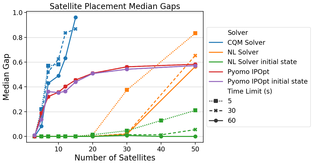
Fig. 35 On all problem sizes tested, D-Wave’s nonlinear solver finds the best solutions to the satellite placement problem with 60-second runtimes.#

Nonlinear Model: Full Formulation#

import itertools
import numpy as np

from dwave.optimization import Model
from dwave.optimization import linprog
from dwave.optimization.mathematical import hstack, vstack, concatenate

model = Model()

D = model.constant(D)
W = model.constant(W)
E = model.constant(E)

num_satellites = W.size()

x = model.list(num_satellites)

d = D[x, :][:, x]
w = W[x]
e = E[x]

# Create a list of all ordered pairs of satellites to construct A
combinations = list(itertools.combinations(range(num_satellites), 2))
num_rows = len(combinations)

from_ = model.constant([i for i, j in combinations])
to_ = model.constant([j for i, j in combinations])

# Construct the part of A indexed by the theta values
theta = np.zeros((num_rows, num_satellites))
for row, (i, j) in enumerate(combinations):
    theta[row][i] = +1
    theta[row][j] = -1
model.theta = theta = model.constant(np.vstack((theta, -theta)))
# Concatenate A with the column for the coefficients of z
d_combinations = d[from_, to_]
A = hstack((theta, concatenate((d_combinations, d_combinations)).reshape(-1, 1)))
b_ub = model.constant([0] * num_rows + [360] * num_rows)

# Create the vectors for the upper and lower bounds
lb = concatenate((w, model.constant([0])))
ub = concatenate((e, model.constant([+1_000])))  # just a large number

# And finally we want to maximize z
c = model.constant([0] * num_satellites + [-1])

# Create the LP
lp = linprog(c=c, A_ub=A, b_ub=b_ub, lb=lb, ub=ub)

# Add the LP as a constraint to the model
success = model.add_constraint(lp.success)
model.minimize(lp.fun)

cntx = model.lock()