Flow-Shop Scheduling#

Flow-shop scheduling (FSS) is an optimization challenge that involves organizing a set of jobs that need to be processed through multiple machines in a specific order. This type of scheduling is important in manufacturing and production environments, where operators are pressed to efficiently manage the workflow by optimizing the time it takes to complete each job and thus maintain a smooth and linear progression through the production line.

Specifically, in the FSS problem, a set of \(n\) jobs each having \(m\) tasks must run in order on \(m\) machines; for example, see Figure 31. The order of the jobs must be consistent across all machines. The goal is to find a permutation of the jobs that minimizes the overall makespan (that is, the finish time).

This study shows how the optimization of flow-shop scheduling using D-Wave’s hybrid nonlinear-program solver (NL solver) improves this process, with the goal of driving operational efficiencies. This study includes performance benchmarks of D-Wave’s NL and CQM solvers as well as COIN-OR, OR-Tools, and SciPy’s HiGHS.

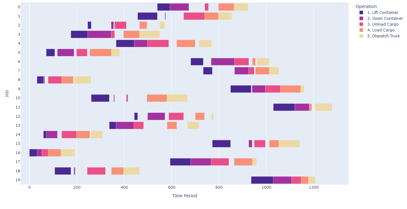
Fig. 31 An example of flow-shop scheduling.#

Mathematical Models#

This section discusses the various mathematical models that were used in this study.

Mixed Integer Linear Programming (MILP) Model#

For MILP solvers, the study uses the formulation provided by Manne [Man1960]. Job orders are represented by binary variables \(x_{ij}\). For each pair of jobs \(i\) and \(j\), the variable \(x_{ij}\) is assigned a value of 1 if job \(i\) is scheduled to be processed after job \(j\). If job \(i\) is not processed after job \(j\), then \(x_{ij}\) is assigned a value of 0. This binary system determines the sequence of job processing. Task completion times are encoded by continuous variables. In the resulting formulation, the number of binary variables is quadratic in the number of jobs, and the number of continuous variables is equal to the number of jobs multiplied by the number of tasks.

The assigned constraints ensure that the jobs do not overlap, and the order of the jobs is respected across all machines. For each job, the number of constraints is quadratic in the number of machines.

This formulation is used by the CQM solver, COIN-OR’s Pulp CBC CMD solver, and SciPy’s HiGHS.

OR-Tools CP-SAT Solver#

OR-Tools defines an FSS formulation that fits their API where task processing times are passed as an \(n\times m\) matrix.

Nonlinear Solver Model#

D-Wave’s NL solver can efficiently encode an FSS problem by taking advantage of a list variable (ListVariable) that encodes an ordering of the jobs. This variable eliminates the need for both the quadratic number of binary variables representing job orders and constraints preserving job order for the MILP formulation. The array of processing times is converted to a constant variable from which the task end times are computed. As a result, there is no need to encode constraints that prevent the jobs from overlapping.

The relevant Python code is as follows:

from dwave.optimization import Model
from dwave.optimization.mathematical import maximum

model = Model()

# Add the constant processing-times matrix
times = model.constant(processing_times)

# The decision symbol is a num_jobs-long array of integer variables
order = model.list(num_jobs)
end_times = []

for machine_m in range(num_machines):
    machine_m_times = []
    if machine_m == 0:
        for job_j in range(num_jobs):
            if job_j == 0:
                machine_m_times.append(times[machine_m, :][order[job_j]])
            else:
                end_job_j = times[machine_m, :][order[job_j]]
                end_job_j += machine_m_times[-1]
                machine_m_times.append(end_job_j)
    else:
        for job_j in range(num_jobs):
            if job_j == 0:
                end_job_j = end_times[machine_m - 1][job_j]
                end_job_j += times[machine_m, :][order[job_j]]
                machine_m_times.append(end_job_j)
            else:
                end_job_j = maximum(end_times[machine_m - 1][job_j], machine_m_times[-1])
                end_job_j += times[machine_m, :][order[job_j]]
                machine_m_times.append(end_job_j)
    end_times.append(machine_m_times)
makespan = end_times[-1][-1]
# The objective is to minimize the last end time
model.minimize(makespan)
cntx = model.lock()

This model is available via the flow_shop_scheduling() generator.

Results#

All problems were run with a time limit of 150 seconds. Results are reported as optimality gaps (that is, (energy/best solution) - 1) when feasible. Infeasible solutions correspond to infinite gaps in the median, and if the median is infeasible, the data point is not shown in the plot. In order to impose time limits on COIN-OR’s solver, presolve techniques are turned off. Presolve modifies the model by removing redundant equations, changing some equations to bounds, and so forth without contributing to the time limit.

D-Wave’s NL solver and CQM solver benchmarks were run on D-Wave’s Leap™ quantum cloud service. COIN-OR, OR-Tools, and HiGHS were run on an Intel Core i9-7900X CPU @ 3.30GHz processor with 16GB RAM. The benchmarks for OR-Tools were run with eight threads (the minimum number for parallel search), and the remaining were run with a single thread. The instances run in this benchmark are the set of Taillard FSS instances [Tai1993], which is an industry-standard benchmarking testbed (for example, [Li2022], [Kar2022], [Mao2021]). These 120 instance files contain the processing times for each task, with problem sizes ranging from 20 to 500 jobs on 5 to 20 machines. For each job size, there are instances with 5, 10, and 20 machines, excluding 200 jobs (having 10 and 20 machines) and 500 jobs (having 20 machines).

Figure 32 shows the results on the Taillard FSS instances with a time limit of 150 seconds. The plot displays the median gap versus number of jobs for each solver. The complete study contains more time limits, where the results are qualitatively the same, except for OR-Tools obtaining optimality in the smallest instances with the largest time limit. For each number of jobs with a 150-second runtime, D-Wave’s NL solver outperforms the other solvers.

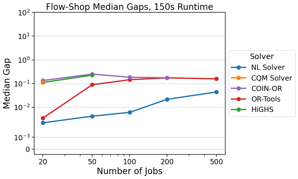
lineplot — Fig. 32 On FSS problems with 150 seconds of runtime, the median gap for solutions found by D-Wave’s NL solver beats the median gaps found by all other solvers tested on all sizes available in the Taillard benchmarking library.#