Quadratic Assignment Problem#

The goal of the quadratic assignment problem (QAP) is to select locations that minimize the total flow cost between facilities.

The optimization tasks for this problem include minimizing transportation costs, reducing travel distances, and optimizing resource allocation. These tasks are commonly found in industries where efficient layout planning and logistics are essential, such as manufacturing, supply chain management, and facility layout design.

In QAP, we are given a set of \(n\) facilities and \(n\) locations. Between each pair of facilities, there is a “flow” (for example, the amount of supplies transported from one facility to the other). The goal is to place the facilities so that the sum of the flows times the distances is minimized. The objective function is nonlinear in the problem variables, which makes it difficult to formulate for MILP and LP solvers.

Fig. 33 The quadratic assignment problem.#

This study shows that on QAP problems from the Taillard benchmarking library (see [Tai1991] and [Tai1995]) with 150 seconds of runtime, the gap for solutions found by D-Wave’s hybrid nonlinear-program solver, or NL solver, beats or ties all “b” and “c” instances. For the “a” instances, the only solver to beat the NL solver is D-Wave’s hybrid constrained quadratic model (CQM) solver.

Problem Instances#

The instances benchmarked for this paper are the Taillard instances ([Tai1991] and [Tai1995]). These 26 problems contain the distance between each pair of locations and the flow between each pair of facilities, with problem sizes ranging from 12 to 256 locations (the number of locations is equal to the number of facilities). These instances, categorized as “a”, “b”, and “c” are as follows:

“a” instances are from [Tai1991] and are uniformly generated.
“b” instances are from [Tai1995] and are randomly generated, with distance matrices containing Euclidean distances between pairs of \(n\) randomly generated points in the plane.
“c” instances are from [Tai1995] and have binary flow matrices with a block of 1s in the upper left corner and are inspired by the problem of printing greys of a given density.

Mathematical Models#

This section discusses the various mathematical models that were used in this study.

Mixed Integer Nonlinear Programming (MINLP) Model#

For MINLP solvers, the study uses binary variables \(x_{ij}\) to indicate whether facility \(i\) is placed in location \(j\). Thus the number of variables is quadratic in the number of locations. If \(F_{ik}\) is the flow from facility \(i\) to facility \(k\), and \(D_{j\ell}\) is the distance between location \(j\) and location \(\ell\), then the aim is to minimize the objective function:

\[\sum_{i,j,k,\ell} F_{ik} D_{j\ell} x_{ij} x_{k\ell}\]

The sum is over all pairs of facilities \(i,j\) and all pairs of locations \(k,\ell\). The formulation also encodes constraints to ensure that there is only one facility placed in each location and only one location per facility. The number of constraints is twice the number of locations.

This formulation is used by D-Wave’s hybrid CQM solver, COIN-OR with Ipopt (Interior Point Optimizer), and OR-Tools with the CP-SAT solver.

SciPy Quadratic Assignment Function#

SciPy provides a quadratic assignment function that includes its 2-opt method, a local search algorithm that searches by swapping facility placements.

Nonlinear Model#

D-Wave’s NL solver can efficiently encode a QAP problem by taking advantage of a list() variable that encodes an ordering of the facility placements. This variable eliminates the need for both the quadratic number of binary variables representing facility placements and the constraints preventing multiple facilities per location (and vice versa) required by the MINLP formulation. The arrays of flows and distances are converted to constant variables from which the objective value is computed.

The relevant Python code is as follows:

from dwave.optimization import Model

model = Model()

# Add the flow and distance matrices
F = model.constant(flows)
D = model.constant(distances)

# Create a list variable to encode facility placement
n = distances.shape[0]
x = model.list(n)

# Minimize the sum of the flows times the distances
model.minimize((F*D[x,:][:,x]).sum())
cntx = model.lock()

This model is available via the quadratic_assignment() generator.

Results#

All problems were run with a time limit of 150 seconds. Results are reported as optimality gaps \(( \frac{\rm energy}{\rm best\: known\: solution} - 1)\) when feasible. Infeasible solutions correspond to infinite gaps in the median, and if the median is infeasible, the data point is not shown in the plot. In order to impose time limits on COIN-OR’s solver, presolve techniques are turned off. Solvers that terminate faster than the time limit are rerun for the full allocated time and the minimum objective value found is saved.

D-Wave’s NL solver and CQM solver benchmarks ran on D-Waves’s Leap™ quantum cloud service. COIN-OR, OR-Tools, and SciPy were run on an Intel Core i9-7900X CPU @ 3.30GHz processor with 16GB RAM. The benchmarks for OR-Tools were run with eight threads, and the remaining were run with a single thread.

Figure 34 shows results on the Taillard QAP instances with a time limit of 150 seconds.

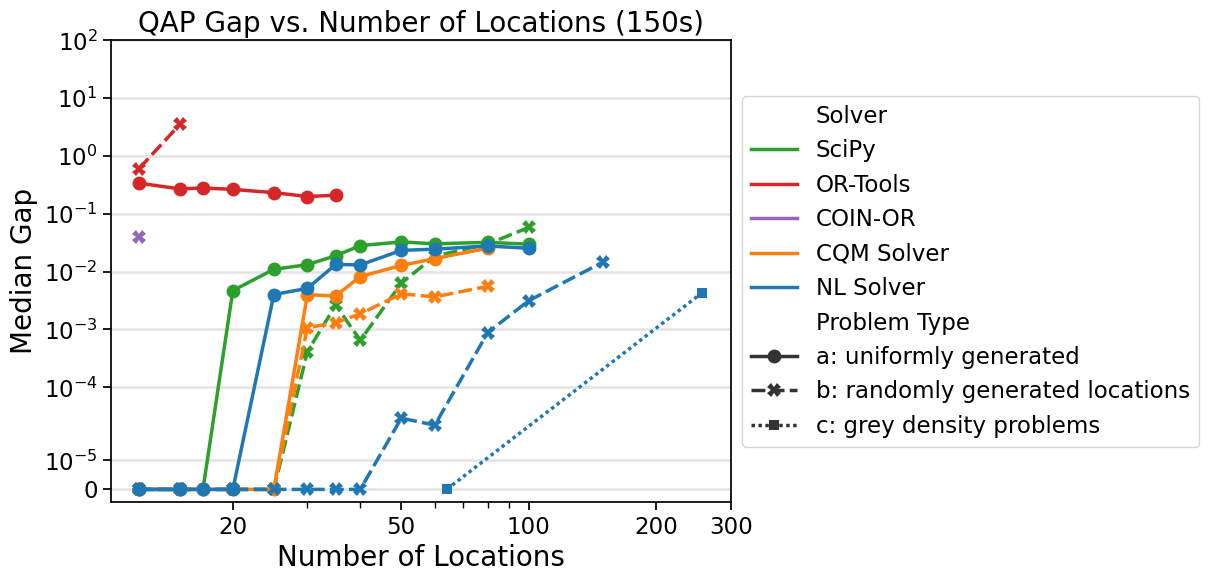
lineplot — Fig. 34 The complete study contains more time limits. For all “b” and “c” instances, the NL solver beats or ties all other solvers. For all “a” instances, the only solver to beat the NL solver is D-Wave’s CQM solver. The NL solver is the only solver able to obtain a feasible solution for the problems of size 150 and 256 for all time limits tested.#