

BQM Solver Parameters#
This section describes the properties of quantum-classical hybrid
binary quadratic model solvers such as the Leap
service’s hybrid_binary_quadratic_model_version2. For the parameters
you can configure, see the BQM Solver Parameters section.
bqm#
Ocean software’s dimod.binary.BinaryQuadraticModel (BQM) contains
linear and quadratic biases for problems formulated as
binary quadratic models as well as additional
information such as variable labels and offset.
Relevant Properties#
maximum_number_of_variables defines the maximum number of problem variables for hybrid solvers.
maximum_number_of_biases defines the maximum number of problem biases for hybrid solvers.
minimum_time_limit and maximum_time_limit_hrs define the runtime duration for hybrid solvers.
Example#
This illustrative example submits a BQM created from a QUBO to a hybrid BQM solver.
>>> from dwave.system import LeapHybridBQMSampler
...
>>> Q = {('x1', 'x2'): 1, ('x1', 'z'): -2, ('x2', 'z'): -2, ('z', 'z'): 3}
>>> bqm = dimod.BQM.from_qubo(Q)
>>> sampleset = LeapHybridBQMSampler().sample(bqm)
h#
For Ising problems, the \(h\) values are the linear coefficients (biases). A problem definition comprises both h and J values.
Because the quantum annealing process minimizes the energy function of the Hamiltonian, and \(h_i\) is the coefficient of variable \(i\), returned states of the problem’s variables tend toward the opposite sign of their biases; for example, if you bias the qubits representing variable \(v_i\) with \(h_i\) values of \(-1\), variable \(v_i\) is more likely to have a final state of \(+1\) in the solution.
For QUBO problems, use Q instead of \(h\) and \(J\); see the Ising-QUBO Transformations section for information on converting between the formulations.
If you are submitting directly through SAPI’s REST API, see the SAPI REST Interface section for more information.
Default is zero linear biases.
Relevant Properties#
maximum_number_of_variables defines the maximum number of problem variables for hybrid solvers.
maximum_number_of_biases defines the maximum number of problem biases for hybrid solvers.
Example#
This example sets linear and quadratic biases for a simple Ising problem.
>>> from dwave.system import LeapHybridBQMSampler
...
>>> h = {'a': 1, 'b': -1}
>>> J = {('a', 'b'): -1}
>>> sampleset = LeapHybridBQMSampler().sample_ising(h, J)
J#
For Ising problems, the \(J\) values are the quadratic coefficients. The larger the absolute value of \(J\), the stronger the coupling between pairs of variables (and qubits on QPU solvers). An Ising problem definition comprises both h and J values.
Because the quantum annealing process minimizes the energy function of the Hamiltonian, and this parameter sets the strength of the couplers between qubits, the following obtains:
\(\textbf {J < 0}\): Ferromagnetic coupling; coupled qubits tend to be in the same state, \((1,1)\) or \((-1,-1)\).
\(\textbf {J > 0}\): Antiferromagnetic coupling; coupled qubits tend to be in opposite states, \((-1,1)\) or \((1,-1)\).
\(\textbf {J = 0}\): No coupling; qubit states do not affect each other.
For QUBO problems, use Q instead of \(h\) and \(J\); see the Ising-QUBO Transformations section for information on converting between the formulations.
If you are submitting directly through SAPI’s REST API, see the SAPI REST Interface section for more information.
Default is zero quadratic biases.
Relevant Properties#
maximum_number_of_variables defines the maximum number of problem variables for hybrid solvers.
maximum_number_of_biases defines the maximum number of problem biases for hybrid solvers.
Example#
This example sets linear and quadratic biases for a simple Ising problem.
>>> from dwave.system import LeapHybridBQMSampler
...
>>> h = {'a': 1, 'b': -1}
>>> J = {('a', 'b'): -1}
>>> sampleset = LeapHybridBQMSampler().sample_ising(h, J)
label#
Problem label you can optionally tag submissions with. You can set as a label a non-empty string of up to 1024 Windows-1252 characters that has meaning to you or is generated by your application, which can help you identify your problem submission. You can see this label on the Leap service’s dashboard and in solutions returned from SAPI.
Example#
This illustrative example sets a label on a submitted problem.
>>> from dwave.system import LeapHybridBQMSampler
...
>>> Q = {('x1', 'x2'): 1, ('x1', 'z'): -2, ('x2', 'z'): -2, ('z', 'z'): 3}
>>> bqm = dimod.BQM.from_qubo(Q)
>>> sampleset = LeapHybridBQMSampler().sample(
...     bqm,
...     label="Simple example")
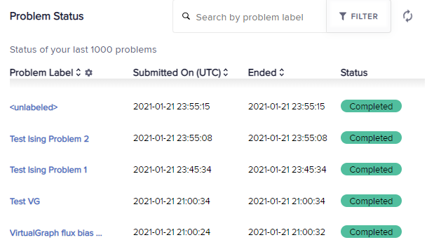
Fig. 24 Problem labels on the dashboard.#
Q#
A quadratic unconstrained binary optimization (QUBO) problem is defined using an upper-triangular matrix, \(\rm \textbf{Q}\), which is an \(N \times N\) matrix of real coefficients, and \(\textbf{x}\), a vector of binary variables. The diagonal entries of \(\rm \textbf{Q}\) are the linear coefficients (analogous to \(h\), in Ising problems). The nonzero off-diagonal terms are the quadratic coefficients that define the strength of the coupling between variables (analogous to \(J\), in Ising problems).
Input may be full or sparse. Both upper- and lower-triangular values can be used; (\(i\), \(j\)) and (\(j\), \(i\)) entries are added together.
If you are submitting directly through SAPI’s REST API, see the SAPI REST Interface section for more information.
Default is zero linear and quadratic biases.
Relevant Properties#
maximum_number_of_variables defines the maximum number of problem variables for hybrid solvers.
maximum_number_of_biases defines the maximum number of problem biases for hybrid solvers.
Example#
This example submits a QUBO to a QPU solver.
>>> from dwave.system import LeapHybridBQMSampler
...
>>> Q = {(0, 0): -3, (1, 1): -1, (0, 1): 2, (2, 2): -1, (0, 2): 2}
>>> sampleset = LeapHybridBQMSampler().sample_qubo(Q)
time_limit#
Specifies the maximum runtime, in seconds, the solver is allowed to work on the given problem. Can be a float or integer.
Default value is problem dependent.
Relevant Properties#
minimum_time_limit defines the range of supported values for a given BQM.
Example#
This illustrative example configures a time limit of 6 seconds.
>>> from dwave.system import LeapHybridBQMSampler
...
>>> Q = {('x1', 'x2'): 1, ('x1', 'z'): -2, ('x2', 'z'): -2, ('z', 'z'): 3}
>>> sampleset = LeapHybridBQMSampler().sample_qubo(
...     Q,
...     time_limit=6)