Model Construction

Nonlinear programming (NLP) is the process of solving an optimization problem where some of the constraints are not linear equalities and/or the objective function is not a linear function. Such optimization problems are pervasive in business and logistics: inventory management, scheduling employees, equipment delivery, and many more.

Nonlinear Models

The dwave-optimization tool enables you to formulate the nonlinear models needed for such industrial optimization problems. The model can then be submitted to the Leap service’s quantum-classical hybrid nonlinear solver (also known as the Stride™ hybrid solver) to find good solutions. The design principles and major features are described in the dwave-optimization philosophy page.

This section explains the nonlinear model and shows how to construct such a model. The Using the Stride Solver section shows how to submit these models for solution. Successful implementation, as for any solver, requires following some best practices in formulating your model.

For other models (e.g., CQM), see the Other Models section.

Symbols

dwave-optimization nonlinear models can be mapped to a directed acyclic graph. The model’s symbols—decision variables, intermediate variables, constants, and mathematical operations—are represented as nodes in the graph while the flow of operations upon these symbols are represented as the graph’s edges.

Fig. 5 A nonlinear model as a directed acyclic graph.

Consider an illustrative problem of finding the minimum of a function of an integer variable, the polynomial \(y = i^2 - 4i\).

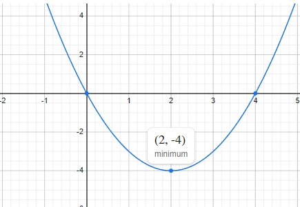
Fig. 6 Minimum point of a simple polynomial, \(y = i^2 - 4i\).

The dwave-optimization package can formulate the problem as nonlinear model as follows:

>>> from dwave.optimization import Model
...
>>> model = Model()
>>> i = model.integer(lower_bound=-5, upper_bound=5)
>>> c = model.constant(4)
>>> y = i**2 - c*i
>>> model.minimize(y)

The code above has the following elements:

• i is a IntegerVariable symbol, typically constructed with the integer() method, that represents a single integer of values between \(-5\) and \(+5\). It is a decision variable: to find the minimum of the polynomial, a solver must assign values to decision variable i such that the objective function of this model is minimized.

• c is a Constant symbol that represents a single invariable value, \(4\), which is the linear coefficient multiplying \(i\) in the polynomial. This type of symbol is used as input to mathematical operations but its value is never updated by a solver.

• y is an intermediate symbol used for convenience to formulate the model in a human-readable way. It is fully determined by other symbols—the i and c symbols—and so implicitly constrained. A solver must update y if it updates i, to a value fully determined by the value it selected to assign to i.

• The Min symbol is a mathematical operation on inputs from other symbols. In this model, it generates the objective function.

The directed acyclic graph below illustratively represents the model for minimizing polynomial \(y = i^2 - 4i\).

Fig. 7 A directed acyclic graph that illustrates one way of representing the model for minimizing polynomial \(y = i^2 - 4i\).

The dwave-optimization package’s to_networkx() method generates the graph that represents the model. The following code uses DAGVIZ to draw the NetworkX graph for the \(y = i^2 - 4i\) polynomial.

>>> import dagviz
...
>>> G = model.to_networkx()
>>> r = dagviz.render_svg(G)
>>> with open("model.svg", "w") as f:
...     f.write(r)

This creates the following image:

Fig. 8 The directed acyclic graph for the model.

The package provides various symbols that enable you to select those most suited to an efficient formulation of your model.

Tip

Scan the symbols section to see supported symbols, and follow the links from a symbol you need to the method used to instantiate it.

States

States represent assignments of values to a symbol. For example, an integer decision variable, represented by an IntegerVariable symbol, of size \(2 \times 3\), might have states

\[\begin{split}\begin{bmatrix} 1 & 1 & 2 \\ 4 & 5 & 5 \end{bmatrix} \text{ and } \begin{bmatrix} 1 & 1 & 3 \\ 4 & 5 & 5 \end{bmatrix}.\end{split}\]

Such states, which might be returned from a solver, represent two assignments that differ in one element of the array (element \((0,2)\)), as is typical at the end of an iterative solution process.

The solutions to nonlinear models you submit to the Leap service’s Stride solver are states of the model’s decision variables. For example, the state of symbol i in the model above for the simple polynomial, \(y = i^2 - 4i\).

The dwave-optimization package enables you to set the states of symbols in a model. You can set states for two purposes:

• Setting initial states for the solver. For some problems you might have estimates or guesses of solutions, and by providing to the solver, as part of your problem submission, such assignments of decision variables as an initial state of the model, you may accelerate the solution.

• Testing and developing your models.

Setting States

A newly created model has a state size of zero. After the Stride solver returns solutions, the model’s state size is the number of states returned for your problem. The following code, as an example of testing, sets a state size of five for the \(y = i^2 - 4i\) polynomial’s model (meaning decision variable i has five assigned solution values).

>>> print(model.states.size())
0
>>> model.states.resize(5)
...
>>> for name, sym in {"i": i, "c": c, "y": y}.items():
...     try:
...         print(f"Variable {name} has value {sym.state(0)} for state 0")
...     except:
...         print(f"Cannot access variable {name}")
Variable i has value 0.0 for state 0
Variable c has value 4.0 for state 0
Cannot access variable y

States for the decision variable have been initialized (to zero for the IntegerVariable of this example), states for the constant symbols have an invariable value, but states of intermediate (successor) symbols, which are implicitly constrained, depend on the states of predecessor symbols; in this example, the state of \(y\) is set based on the states of \(i\) and \(c\). This is calculated only when the model is locked using the lock() method.

>>> with model.lock():
...     print(f"Variable y has value {y.state(0)} for state 0")
Variable y has value 0.0 for state 0

The following code sets values for states 0 to 4 of decision variable i and prints the resulting value of the model’s objective function for each state.

>>> with model.lock():
...     for indx in range(model.states.size()):
...         i.set_state(indx, [indx])
...         print(f"For state {indx}, i={i.state(indx)} results in objective {model.objective.state(indx)}")
For state 0, i=0.0 results in objective 0.0
For state 1, i=1.0 results in objective -3.0
For state 2, i=2.0 results in objective -4.0
For state 3, i=3.0 results in objective -3.0
For state 4, i=4.0 results in objective 0.0

Accessing States

The code above selects a symbol by label (’i’); however, you can also select symbols in a model without using labels. Use the iter_decisions() method to iterate over a model’s decision variables, or the iter_symbols() and iter_constraints() methods for all the model’s symbols and constraints. The \(y = i^2 - 4i\) polynomial’s model has just one decision variable:

>>> with model.lock():
...     model.states.resize(1)
...     decision_var = next(model.iter_decisions())
...     decision_var.set_state(0, [2])
...     print(model.objective.state(0))
-4.0

This process of iterating through a model to select symbols of various types (decision variables, constraints, etc) is helpful when constructing the model is separated from submitting the model to a solver for solutions, for example in a production application or when using the package’s model generators.

You might use a generator for a bin packing problem, bin_packing(), for example, to find the smallest number of bins that can hold a set of weighted items, given that each bin has a weight capacity:

>>> from dwave.optimization.generators import bin_packing
>>> model = bin_packing([3, 5, 1, 3], 7)

Thees two lines of code instantiate a model for packing four items with various weights into bins with maximum capacity 7. With a generator, in contrast to a model you construct before using, you might not have direct access to its variables to inspect states. You can submit the model to the Stride solver, as shown in the Using the Stride Solver section, and the solver sets some number of states in the model. To see these returned solutions, you select the model’s decision variable with the iter_decisions() method.

>>> items = next(model.iter_decisions())

Constructing Models

Typically, you construct your model by instantiating decision-variable symbols, using such model methods as integer() and set(), and constants (constant()). You then perform operations on these symbols, using functions such as matrix multiplication, matmul(), creating successor symbols. In this way you formulate objectives and constraints. You can use the minimize() method to specify the symbol representing an objective to optimize for.

You can create a model for the traveling salesperson problem using the list() method to instantiate a ListVariable symbol, as the decision variable, and the constant() method to hold a distance matrix as a Constant symbol. The list decision variable is used for this problem because any itinerary of cities, each visited once, is a permutation of the cities to be visited (with each city represented by an integer).[1]

>>> from dwave.optimization import Model
...
>>> model = Model()
>>> ordered_cities = model.list(3)          # decision variable
>>> DM = model.constant([                   # constant distance matrix
...     [0, 3, 1],
...     [1, 0, 3],
...     [3, 1, 0]])

[1]

The Building Good Models section discusses how to select decision variables.

Such decision-variable symbols and constant symbols form the “root” of the directed acyclic graph underlying the model.

Fig. 9 A directed acyclic graph that shows a single decision variable, ordered_cities, represented by a ListVariable symbol, and a constant, DM, represented by a Constant symbol, which holds the distance matrix.

Typically, you add symbols to the model through mathematical operations between symbols. The BasicIndexing symbol, for example, is created by operations similar to those of NumPy’s basic indexing. These symbols are successors of the root symbols on the directed acyclic graph, and form part of the mathematical formulation.

>>> from_city = ordered_cities[:-1]
>>> to_city = ordered_cities[1:]
>>> first_city = ordered_cities[0]
>>> last_city = ordered_cities[-1]

Fig. 10 A directed acyclic graph that shows the root symbols at the bottom and the BasicIndexing symbols above those.

You can access these symbols by iterating on the model’s symbols.

>>> with model.lock():
...     for symbol in model.iter_symbols():
...         print(f"Symbol {type(symbol)} is node {symbol.topological_index()}")
Symbol <class 'dwave.optimization.symbols.collections.ListVariable'> is node 0
Symbol <class 'dwave.optimization.symbols.constants.Constant'> is node 1
Symbol <class 'dwave.optimization.symbols.indexing.BasicIndexing'> is node 2
Symbol <class 'dwave.optimization.symbols.indexing.BasicIndexing'> is node 3
Symbol <class 'dwave.optimization.symbols.indexing.BasicIndexing'> is node 4
Symbol <class 'dwave.optimization.symbols.indexing.BasicIndexing'> is node 5

The AdvancedIndexing symbol is created by operations similar to those of NumPy’s advanced indexing. It is used here to represent the distances between cities for the selected itinerary and the distance to return from the last city to the first.

>>> itinerary = DM[from_city, to_city]
>>> return_to_origin = DM[last_city, first_city]

Fig. 11 A directed acyclic graph that shows the root symbols at the bottom and the BasicIndexing and AdvancedIndexing symbols above those.

Next, sum the distances. Note that the total sum uses the + operation, which is equivalent to the add() function.

>>> distance_itinerary = itinerary.sum()
>>> distance_return = return_to_origin.sum()
>>> distance_total = distance_itinerary + distance_return

Fig. 12 A directed acyclic graph that shows the root symbols at the bottom, the BasicIndexing and AdvancedIndexing symbols above those, and the Sum and Add symbols.

Finally, you can define the objective, which is to minimize the distance traveled.

>>> model.minimize(distance_total)

Using the same few lines of code as in the Symbols section above, you can draw the graph of the model.

Fig. 13 The directed acyclic graph for the model.

You can now submit the model to the Stride solver or test it. Here, all permutations of a ListVariable decision variable of length three are tested.

>>> import itertools
...
>>> list_values = [0, 1, 2]
>>> with model.lock():
...     model.states.resize(1)
...     for solution in itertools.permutations(list_values):
...         ordered_cities.set_state(0, solution)
...         print(f"Itinerary {solution} has distance {distance_total.state(0)}")
Itinerary (0, 1, 2) has distance 9.0
Itinerary (0, 2, 1) has distance 3.0
Itinerary (1, 0, 2) has distance 3.0
Itinerary (1, 2, 0) has distance 9.0
Itinerary (2, 0, 1) has distance 9.0
Itinerary (2, 1, 0) has distance 3.0

In practice, you would likely code such a model with fewer labeled symbols.

>>> from dwave.optimization import Model
...
>>> model = Model()
>>> ordered_cities = model.list(3)
>>> DM = model.constant([
...     [0, 3, 1],
...     [1, 0, 3],
...     [3, 1, 0]])
>>> itinerary = DM[ordered_cities[:-1], ordered_cities[1:]]
>>> return_to_origin = DM[ordered_cities[-1], ordered_cities[0]]
>>> distance_total = itinerary.sum() + return_to_origin.sum()
>>> model.minimize(distance_total)

You might even use an existing generator, such as the traveling_salesperson() generator, in which case you have no labels at all.

>>> from dwave.optimization.generators import traveling_salesperson
...
>>> DM = [[0, 3, 1], [1, 0, 3], [3, 1, 0]]
>>> model = traveling_salesperson(distance_matrix=DM)

In such cases, you access the model’s states using the iter_decisions(), iter_symbols(), and iter_constraints() methods.

>>> with model.lock():
...     model.states.resize(1)
...     itinerary = next(model.iter_decisions())
...     itinerary.set_state(0, [0, 2, 1])
...     print(f"Objective is {model.objective.state(0)}")
Objective is 3.0

Successful implementation, as for any solver, requires following some best practices in formulating your model: see the Building Good Models for guidance.

Other Models

This section provides examples of creating quadratic models that can then be solved on a Leap service hybrid solver such as the CQM solver. Typically you construct a model when reformulating your problem, using such techniques as those presented in the Reformulating a Problem section.

The dimod package provides a variety of model generators. These are especially useful for testing code and learning.

CQM Example: Using a dimod Generator

This example creates a CQM representing a knapsack problem of ten items.

>>> cqm = dimod.generators.random_knapsack(10)

CQM Example: Symbolic Formulation

This example constructs a CQM from symbolic math, which is especially useful for learning and testing with small CQMs.

>>> x = dimod.Binary('x')
>>> y = dimod.Integer('y')
>>> cqm = dimod.CQM()
>>> objective = cqm.set_objective(x+y)
>>> cqm.add_constraint(y <= 3)
'...'

For very large models, you might read the data from a file or construct from a NumPy array.

BQM Example: Using a dimod Generator

This example generates a BQM from a fully-connected graph (a clique) where all linear biases are zero and quadratic values are uniformly selected -1 or +1 values.

>>> bqm = dimod.generators.random.ran_r(1, 7)

BQM Example: Python Formulation

For learning and testing with small models, construction in Python is convenient.

The maximum cut problem is to find a subset of a graph’s vertices such that the number of edges between it and the complementary subset is as large as possible.

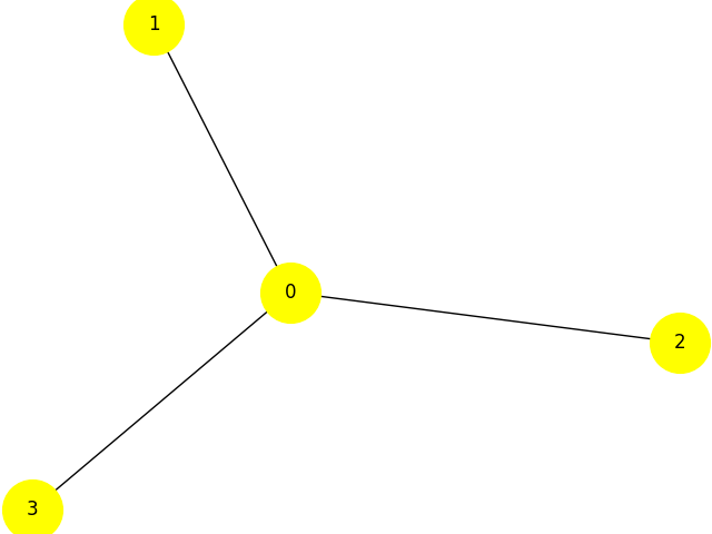
Fig. 14 Star graph with four nodes.

The dwave-examples Maximum Cut example demonstrates how such problems can be formulated as QUBOs:

\[\begin{split}Q = \begin{bmatrix} -3 & 2 & 2 & 2\\ 0 & -1 & 0 & 0\\ 0 & 0 & -1 & 0\\ 0 & 0 & 0 & -1 \end{bmatrix}\end{split}\]

>>> qubo = {(0, 0): -3, (1, 1): -1, (0, 1): 2, (2, 2): -1,
...         (0, 2): 2, (3, 3): -1, (0, 3): 2}
>>> bqm = dimod.BQM.from_qubo(qubo)

BQM Example: Construction from NumPy Arrays

For performance, especially with very large BQMs, you might read the data from a file using methods, such as from_file() or from NumPy arrays.

This example creates a BQM representing a long ferromagnetic loop with two opposite non-zero biases.

>>> import numpy as np
>>> linear = np.zeros(1000)
>>> quadratic = (np.arange(0, 1000), np.arange(1, 1001), -np.ones(1000))
>>> bqm = dimod.BinaryQuadraticModel.from_numpy_vectors(linear, quadratic, 0, "SPIN")
>>> bqm.add_quadratic(0, 10, -1)
>>> bqm.set_linear(0, -1)
>>> bqm.set_linear(500, 1)
>>> bqm.num_variables
1001

QM Example: Interaction Between Integer Variables

This example constructs a QM with an interaction between two integer variables.

>>> qm = dimod.QuadraticModel()
>>> qm.add_variables_from('INTEGER', ['i', 'j'])
>>> qm.add_quadratic('i', 'j', 1.5)

Additional Examples

• The Basic QPU Examples and Basic Hybrid Examples sections have examples of using QPU solvers and Leap service hybrid solvers on quadratic models.

• The dwave-examples GitHub repository provides more examples.